Intro to Variant Call Format
Overview
Teaching: 30 min
Exercises: 5 minQuestions
How are genotypes and metadata stored in a VCF?
Objectives
Describe the purpose of FORMAT and INFO fields.
Describe what the rows and columns of a VCF represent.
In the setup, you downloaded a compressed VCF file and saved it to
your data directory. Depending on your operating system and what you have
installed, you may be able to preview it from your “Terminal” tab with the
following code. If zless is not available, don’t worry, since everything
else we do will happen in R. To quit zless, type q.
zless data/hmp_agpv4_chr1_subset.vcf.bgz
##fileformat=VCFv4.1
##fileDate=20201110
##HapMapVersion="3.2.1"
##FILTER=All filters passed
##FORMAT=<ID=GT,Number=1,Type=String,Description="Genotype">
##FORMAT=<ID=AD,Number=.,Type=Integer,Description="Allelic depths for the reference and alternate alleles in the order listed">
##FORMAT=<ID=GL,Number=.,Type=Integer,Description="Genotype likelihoods for 0/0, 0/1, 1/1, or  0/0, 0/1, 0/2, 1/1, 1/2, 2/2 if 2 alt alleles">
##INFO=<ID=DP,Number=1,Type=Integer,Description="Total Depth">
##INFO=<ID=NZ,Number=1,Type=Integer,Description="Number of taxa with called genotypes">
##INFO=<ID=AD,Number=.,Type=Integer,Description="Total allelelic depths in order listed starting with REF">
##INFO=<ID=AC,Number=.,Type=Integer,Description="Numbers of ALT alleles in order listed">
##INFO=<ID=AQ,Number=.,Type=Integer,Description="Average phred base quality for alleles in order listed starting with REF">
##INFO=<ID=GN,Number=.,Type=Integer,Description="Number of taxa with genotypes AA,AB,BB or AA,AB,AC,BB,BC,CC if 2 alt alleles">
##INFO=<ID=HT,Number=1,Type=Integer,Description="Number of heterozygotes">
##INFO=<ID=EF,Number=.,Type=Float,Description="EF=het_frequency/(presence_frequency * minor_allele_frequency), if 2 alt alleles,EF for AB,AC,BC pairsis given; from 916 taxa of HapMap 3.1.1">
##INFO=<ID=PV,Number=.,Type=Float,Description="p-value from segregation test between AB or AB, AC, BC if 2 alt alleles, from 916 taxa of HapMap 3.1.1">
##INFO=<ID=MAF,Number=1,Type=Float,Description="Minor allele frequency">
##INFO=<ID=MAF0,Number=1,Type=Float,Description="Minor allele frequency from unimputed HapMap 3.2.1 on 1210 taxa">
##INFO=<ID=IBD1,Number=0,Type=Flag,Description="only one allele present in IBD contrasts; based on 916 taxa of HapMap3.1.1">
##INFO=<ID=LLD,Number=0,Type=Flag,Description="Site in local LD with GBS map (from 916 taxa of HapMap 3.1.1)">
##INFO=<ID=NI5,Number=0,Type=Flag,Description="Site with 5bp of a putative indel from 916 taxa of HapMap 3.1.1">
##INFO=<ID=INHMP311,Number=0,Type=Flag,Description="Site peresent in HapMap3.1.1">
##INFO=<ID=ImpHomoAccuracy,Number=1,Type=Float,Description="Fraction of homozygotes imputed back into homozygotes">
##INFO=<ID=ImpMinorAccuracy,Number=1,Type=Float,Description="Fraction of minor allele homozygotes imputed back into minor allelel homozygotes">
##INFO=<ID=DUP,Number=0,Type=Flag,Description="Site with heterozygotes frequency > 3%">
##ALT=<ID=DEL,Description=Deletion>
##ALT=<ID=INS,Description=Insertion>
##contig=<ID=1,assembly="1">
#CHROM  POS     ID      REF     ALT     QUAL    FILTER  INFO    FORMAT  2005-4  207     32      5023    680     68139   697     75-14gao        764     78004   78551S  792     83IBI3  8982    9058    98F1    B4      B7      B73     B76     B8      B97     BKN009  BKN011  BKN017  BKN018  BKN027  BKN029  C521    CAUMo17 chang69 chang7daxian1   CML103  CML103-run248   CML411  CN104   Co109   CT109   D1139   D20     D23     D801    D857    D892    dai6    DM07    dupl-478        E588    E601    F7584   F939    FR14    fu8538  H114    H84     HD568   hua160  huangchanga     huotanghuang17  Il14H   ji63    K22     Ki11    Ky21    LD61    LH1     LH128   LH190   LH202   LH51    LH60    lian87  liao2204        LP1     luyuan133       Lx9801  M3736   MBUB    Ms71    mu6     N138    N192    N42     NC268   NC358   ning24  ning45  NS501   Oh40B   Pa91    PHG50   PHG83   PHJ31   PHJ75   PHK05   PHM10   PHN11   PHNV9   PHP02   PHR58
   PHT77   PHW17   PHW52   PHWG5   qiong51 R1656   RS710   SC24-1  SG17    shangyin110-1   shen142 SS99    SZ3     tai184  TIL01-JD        TIL03   TIL09   Timpunia-1      VL056883
VL062784        W117    W238    W344    W499    W668    W968    W9706   wenhuang31413   WIL900  wu312   XF117   y9961   yan38   Yd6     ye107   ye8112  yue39-4 yue89A12-1      zhangjin6
       MAIdgiRAPDIAAPEI-12     MAIdgiRAVDIAAPEI-4      MAIdgiRCKDIAAPEI-9      ZEAhwcRAXDIAAPE ZEAxppRALDIAAPEI-9      ZEAxppRAUDIAAPEI-1      ZEAxppRBFDIAAPEI-3      ZEAxppRBMDIAAPEI-6
      ZEAxppRCODIAAPEI-9      ZEAxppRDLDIAAPEI-2      ZEAxujRBADIAAPE 282set_A556     282set_A619     282set_A634     282set_A654     282set_A659     282set_A661     282set_A679     282set_B103     282set_CH701-30 282set_CI187-2  282set_CI31A    282set_CI64     282set_CM7      282set_CML14    282set_CML154Q  282set_CML254   282set_CML287   282set_GT112    282set_H99
282set_I29      282set_IDS28    282set_Ki21     282set_KY228    282set_MS153    282set_Mt42     282set_NC222    282set_NC264    282set_NC338    282set_NC346    282set_NC360    282set_NC366    282set_OH7B     282set_Os420    282set_Pa875    282set_Sg1533   282set_T232     282set_T234     282set_Tx601    282set_Tzi25    282set_Tzi8     282set_VA102    282set_Va14     282set_Va26     282set_W117Ht   282set_Wf9      german_Mo17     german_Lo11     german_FF0721H-7        german_F03802   german_EZ5
1       21000162        1-20689192      G       T       .       PASS    DP=853;NZ=1203;AD=844,9;AC=14;AQ=34,34;GN=1195,2,6;HT=2;EF=1;PV=0.001;MAF=0.006;MAF0=0.02;IBD1;ImpHomoAccuracy=0.983941605839416;ImpMinorAccuracy=0     GT:AD:GL        0/0::   0/0::   0/0:1,0:0,3,28  0/0:2,0:0,6,55  0/0::   0/0::   0/0::   0/0:1,0:0,3,28  0/0::   0/0::   0/0:6,0:0,18,166        0/0::
   0/0::   0/0::   0/0:1,0:0,3,28  0/0:3,0:0,9,83  0/0::   0/0::   0/0:1,0:0,3,28  0/0::   0/0::   0/0::   0/0::   0/0:2,0:0,6,55  0/0::   0/0::   0/0::   0/0::   0/0:1,0:0,3,28  0/0::
0/0:1,0:0,3,28  0/0::   0/0:5,0:0,15,139        0/0:21,0:0,63,583       0/0:1,0:0,3,28  0/0::   0/0::   0/0::   0/0:5,0:0,15,139        0/0::   0/0:2,0:0,6,55  0/0::   0/0::   0/0::   0/0:3,0:0,9,83  0/0::   0/0:1,0:0,3,28  0/0::   0/0::   0/0::   0/0:1,0:0,3,28  0/0::   0/0:1,0:0,3,28  0/0::   0/0::   0/0::   0/0::   ./.::   0/0:1,0:0,3,28  0/0::   0/0:4,0:0,12,111
        0/0::   0/0::   0/0::   0/0::   0/0::   0/0::   0/0:5,0:0,15,139        0/0:4,0:0,12,111        0/0::   0/0:1,0:0,3,28  0/0::   0/0::   0/0::   0/0::   0/0:1,0:0,3,28  0/0::   0/0::   0/0::   0/0::   0/0::   0/0::   0/0::   0/0:6,0:0,18,166        0/0:2,0:0,6,55  0/0:2,0:0,6,55  0/0::   0/0::   0/0:3,0:0,9,83  0/0::   0/0::   0/0::   0/0::   0/0::   0/0::   0/0:1,0:0,3,28  0/0::   0/0::   0/0::   0/0:1,0:0,3,28  0/0::   0/0::   0/0::   0/0:1,0:0,3,28  0/0::   0/0::   0/0::   0/0:2,0:0,6,55  0/0::   0/0::   0/0::   0/0::   0/0:1,0:0,3,28  0/0::   0/0:2,0:0,6,55  0/0::   0/0:1,0:0,3,28  0/0:1,0:0,3,28  0/0:1,0:0,3,28  0/0::   0/0:3,0:0,9,83  0/0::   0/0::   0/0::   0/0:4,0:0,12,111        0/0:1,0:0,3,28  0/0:2,0:0,6,55  0/0:1,0:0,3,28  0/0:1,0:0,3,28  0/0:1,0:0,3,28  0/0::   0/0:1,0:0,3,28  0/0::   0/0::   0/0::   0/0:4,0:0,12,111        0/0:2,0:0,6,55  0/0:2,0:0,6,55  0/0::   0/0:9,0:0,27,250        0/0::   0/0:1,0:0,3,28  0/0::   0/0::   0/0::   0/0:6,0:0,18,166        0/0::   0/0::   0/0:1,0:0,3,28  0/0:5,0:0,15,139        0/0::   0/0:2,0:0,6,55  0/0::   0/0:2,0:0,6,55  0/0::   0/0::   0/0::   0/0::   0/0::   0/0::   0/0::   0/0::   0/0::   0/0:1,0:0,3,28  0/0::   0/0::   0/0::   0/0::   0/0:2,0:0,6,55  0/0::   0/0::   0/0::   0/0::   0/0::   0/0::   0/0::   0/1:2,1:19,0,46 0/0::   0/0::   0/0:1,0:0,3,28  0/0:3,0:0,9,83  0/0::   0/0::   0/0:1,0:0,3,28  0/0::   0/0:1,0:0,3,28  0/0::   0/0::   0/0:1,0:0,3,28  0/0::   0/0::   0/0::   0/0:2,0:0,6,55  0/0::   0/0:3,0:0,9,83  0/0::   0/0:2,0:0,6,55  0/0::   0/0::   0/0::
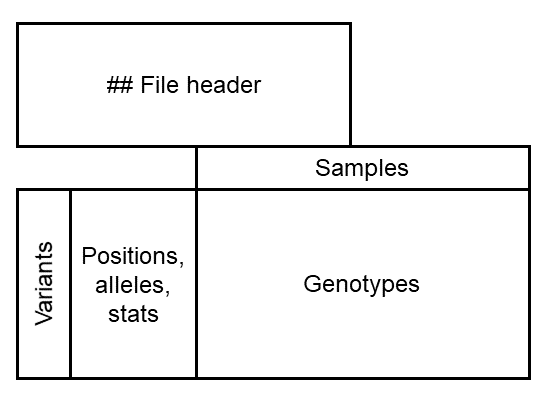
Wow, that’s a lot to look at. What is the information that we have here?
Below is a diagram of the file to make it a bit easier to digest. We have a header, followed by a table of genotypes.
The header
We start with a set of lines beginning with ##. Although these lines aren’t
the most human-readable, if you start looking at the quoted descriptions you’ll
see that the file is “self-documenting”, i.e. there are explanations of what
everything means. We have the date the file was made. The genotype is stored
in a field called GT. DP stores read depth, and MAF stores minor allele
frequency. Many of these are standard fields that are described in the
file format specification.
Others are custom fields, which is why it’s especially helpful to have
descriptions right in the file.
FORMAT fields
We have three fields here tagged as FORMAT: GT, AD, and GL. Anything
with the FORMAT tag indicates information that is stored at the genotype
level, meaning that this is information available for every sample at every
variant.
GT is the genotype. The reference allele is represented by 0, and the
first alternate allele is represented by 1. If there are multiple alleles,
they are represented by numbers 2 and up. (For SNPs, multiple alleles are
rare, but VCF allows any type of variant.) Usually there is a forward slash
between alleles, like 0/0 for a homozygote for the reference allele, or
0/1 for a heterozygote. If genotypes are phased, a pipe is used, so genotypes
might look like 0|0. Polyploid genotypes are allowed, for example 0/0/0/1
for a tetraploid. Missing data are represented by one period for each allele,
for example ./. for diploid data.
AD indicates the sequence read depth for each allele. These are separated by
commas. For example, a homozygous genotype 0/0 might have depths of 5,0
indicating five reads of the reference allele and no reads of the alternative
allele. A heterozygous genotype 0/1 might have depths of 7,4 to indicate
seven reads of the reference allele and four reads of the alternative allele.
Having the read depths allows you to re-do the genotype calling and evaluate
genotype quality yourself.
GL is genotype likelihood (the probability of the observed read depth
distribution, given a genotype), scaled using log10. For a diploid with two
alleles, we’ll see three values, one for 0/0, one for 0/1, and one for
1/1. For example above we see 0,9,83, indicating that 0/0 is very
likely, 0/1 is unlikely but possible, and 1/1 is extremely unlikely. The
reason why there is any uncertainty in the genotype calls is that there could
be sequencing error or undersampling of alleles. There are other fields that
can define this genotype uncertainty including GP, PL, and PP, described in the
file format specification.
These values can be useful for analyses such as GWAS that might want to weight
genotypes by their certainty.
INFO fields
Here we have quite a lot of fields tagged as INFO. The AC field is
described in the file format specification, but all others here are custom.
Each INFO field represents a statistic that was calculated for each variant.
For example, here MAF contains the minor allele frequency. You might use
these fields for filtering markers.
Column headers
After the file header, you should see a row that starts with #CHROM. These
are the column headers for the genotype table. The first nine columns are
always the same:
CHROM: Which chromosome the variant is on.POS: The position (or starting position) of the variant on the chromosome.ID: The name of the variant.REF: The reference allele (the nucleotide matching the reference sequence at this position).ALT: One or more alternative alleles.QUAL: Marker quality. Left as missing (.) by many programs.FILTER: Whether or not the marker passed a filtering step.INFO: Any additional statistics from theINFOfields.FORMAT: WhichFORMATfields are used to code the genotypes, and in what order. This is generally the same for every marker in the dataset, but doesn’t have to be.
After that, there is one column for each sample. In this case the first sample
is called 2005-4. There are no other custom columns, so any custom
information goes into INFO.
Variant rows
Now, the rest of the file is one row per variant. In the first row we see:
- The chromosome is 1.
- The position is 21000162.
- The SNP is named 1-20689192 (after a position in an earlier version of the genome).
- The reference allele is
Gand the alternative allele isT. - No quality score is recorded, and this SNP passed filtering.
- We have a lot of statistics in the
INFOcolumn, separated by semi-colons. - The format is
GT:AD:GL, so that is what we will expect to see for the genotype of each sample. - Under each sample, we see the genotype, allele depths, and genotype likelihoods, separated by colons. Many of these genotypes were imputed and therefore are missing depths and likelihoods.
Once we import this data into R, it will be much more accessible. In the next episode we will cover generally how genomic data and experimental results are stored in BioConductor, which will lead into how we can import and manipulate a VCF.
Discussion
Which FORMAT and INFO fields would you want to use for your analysis, and why? Is there any other information from the VCF that you would use?
Key Points
A VCF is a table with samples in columns and SNPs (or other variants) in rows.
FORMAT fields contain variant-by-sample data pertaining to genotype calls.
INFO fields contain statistics about each variant.
Bioconductor basics
Overview
Teaching: 50 min
Exercises: 15 minQuestions
What are the Bioconductor classes for the types of data we would find in a VCF?
Objectives
Create a GRanges object to indicate regions of the genome that you are interested in.
Load DNA sequences from a reference genome.
Extract assay metadata from the results of an experiment.
Find help pages to learn more about what you can do with this data.
Bioconductor packages are all designed to work together. This is why, when you tried installing five packages, it probably installed dozens of dependencies. The benefit is that the same functions are useful across many different bioinformatics workflows. To explore those building blocks, we’ll load a few of those dependencies.
library(GenomicRanges)
library(Biostrings)
library(Rsamtools)
library(SummarizedExperiment)
We’ll also load magrittr to make some code more readable.
library(magrittr)
Reference genome
In the setup, you downloaded and unzipped a reference genome file.
ref_file <- "data/Zm-B73-REFERENCE-GRAMENE-4.0.fa"
You should build an index for the file. This is another file, ending in
.fai, that indicates where in the file each chromosome starts. It enables
quick access to specific regions of the genome.
indexFa(ref_file)
Now we can import the reference genome.
mygenome <- FaFile(ref_file)
If we try to print it out:
mygenome
class: FaFile
path: data/Zm-B73-REFERENCE-GRAMENE-4.0.fa
index: data/Zm-B73-REFERENCE-GRAMENE-4.0.fa.fai
gzindex: data/Zm-B73-REFERENCE-GRAMENE-4.0.fa.gzi
isOpen: FALSE
yieldSize: NA
Hmm, we don’t see any DNA sequences, just names of files. We haven’t actually loaded the data into R, just told R where to look when we want the data. This saves RAM since we don’t usually need to analyze the whole genome at once.
We can get some information about the genome:
seqinfo(mygenome)
Seqinfo object with 266 sequences from an unspecified genome:
  seqnames      seqlengths isCircular genome
  Chr10          150982314       <NA>   <NA>
  Chr1           307041717       <NA>   <NA>
  Chr2           244442276       <NA>   <NA>
  Chr3           235667834       <NA>   <NA>
  Chr4           246994605       <NA>   <NA>
  ...                  ...        ...    ...
  B73V4_ctg253       82972       <NA>   <NA>
  B73V4_ctg254       69595       <NA>   <NA>
  B73V4_ctg255       46945       <NA>   <NA>
  B73V4_ctg2729     124116       <NA>   <NA>
  Pt                140447       <NA>   <NA>
There are chromosomes, and some smaller contigs.
Challenge: Chromosome names
Look at the help page for
seqinfo. Can you find a way to view all of the sequence names?Solution
There is a
seqnamesfunction. It doesn’t work directly on aFaFileobject however. It works on theSeqInfoobject returned byseqinfo.seqnames(seqinfo(mygenome))[1] "Chr10" "Chr1" "Chr2" "Chr3" [5] "Chr4" "Chr5" "Chr6" "Chr7" [9] "Chr8" "Chr9" "B73V4_ctg1" "B73V4_ctg2" [13] "B73V4_ctg3" "B73V4_ctg4" "B73V4_ctg5" "B73V4_ctg6" [17] "B73V4_ctg7" "B73V4_ctg8" "B73V4_ctg9" "B73V4_ctg10" [21] "B73V4_ctg11" "B73V4_ctg12" "B73V4_ctg13" "B73V4_ctg14" [25] "B73V4_ctg15" "B73V4_ctg16" "B73V4_ctg17" "B73V4_ctg18" [29] "B73V4_ctg19" "B73V4_ctg20" "B73V4_ctg21" "B73V4_ctg22" [33] "B73V4_ctg23" "B73V4_ctg24" "B73V4_ctg25" "B73V4_ctg26" [37] "B73V4_ctg27" "B73V4_ctg28" "B73V4_ctg29" "B73V4_ctg30" [41] "B73V4_ctg31" "B73V4_ctg32" "B73V4_ctg33" "B73V4_ctg34" [45] "B73V4_ctg35" "B73V4_ctg36" "B73V4_ctg37" "B73V4_ctg38" [49] "B73V4_ctg39" "B73V4_ctg40" "B73V4_ctg41" "B73V4_ctg42" [53] "B73V4_ctg43" "B73V4_ctg44" "B73V4_ctg45" "B73V4_ctg46" [57] "B73V4_ctg47" "B73V4_ctg48" "B73V4_ctg49" "B73V4_ctg50" [61] "B73V4_ctg51" "B73V4_ctg52" "B73V4_ctg53" "B73V4_ctg54" [65] "B73V4_ctg56" "B73V4_ctg57" "B73V4_ctg58" "B73V4_ctg59" [69] "B73V4_ctg60" "B73V4_ctg61" "B73V4_ctg62" "B73V4_ctg63" [73] "B73V4_ctg64" "B73V4_ctg65" "B73V4_ctg66" "B73V4_ctg67" [77] "B73V4_ctg68" "B73V4_ctg69" "B73V4_ctg70" "B73V4_ctg71" [81] "B73V4_ctg72" "B73V4_ctg73" "B73V4_ctg74" "B73V4_ctg75" [85] "B73V4_ctg76" "B73V4_ctg77" "B73V4_ctg78" "B73V4_ctg79" [89] "B73V4_ctg80" "B73V4_ctg81" "B73V4_ctg82" "B73V4_ctg83" [93] "B73V4_ctg84" "B73V4_ctg85" "B73V4_ctg86" "B73V4_ctg87" [97] "B73V4_ctg88" "B73V4_ctg89" "B73V4_ctg90" "B73V4_ctg91" [101] "B73V4_ctg92" "B73V4_ctg93" "B73V4_ctg94" "B73V4_ctg95" [105] "B73V4_ctg96" "B73V4_ctg97" "B73V4_ctg98" "B73V4_ctg99" [109] "B73V4_ctg100" "B73V4_ctg101" "B73V4_ctg102" "B73V4_ctg103" [113] "B73V4_ctg104" "B73V4_ctg105" "B73V4_ctg106" "B73V4_ctg107" [117] "B73V4_ctg108" "B73V4_ctg109" "B73V4_ctg110" "B73V4_ctg111" [121] "B73V4_ctg112" "B73V4_ctg113" "B73V4_ctg114" "B73V4_ctg115" [125] "B73V4_ctg116" "B73V4_ctg117" "B73V4_ctg118" "B73V4_ctg119" [129] "B73V4_ctg120" "B73V4_ctg121" "B73V4_ctg122" "B73V4_ctg123" [133] "B73V4_ctg124" "B73V4_ctg125" "B73V4_ctg126" "B73V4_ctg127" [137] "B73V4_ctg128" "B73V4_ctg129" "B73V4_ctg130" "B73V4_ctg131" [141] "B73V4_ctg132" "B73V4_ctg133" "B73V4_ctg134" "B73V4_ctg135" [145] "B73V4_ctg136" "B73V4_ctg137" "B73V4_ctg138" "B73V4_ctg139" [149] "B73V4_ctg140" "B73V4_ctg141" "B73V4_ctg142" "B73V4_ctg143" [153] "B73V4_ctg144" "B73V4_ctg145" "B73V4_ctg146" "B73V4_ctg147" [157] "B73V4_ctg148" "B73V4_ctg149" "B73V4_ctg150" "B73V4_ctg151" [161] "B73V4_ctg152" "B73V4_ctg153" "B73V4_ctg154" "B73V4_ctg155" [165] "B73V4_ctg156" "B73V4_ctg157" "B73V4_ctg158" "B73V4_ctg159" [169] "B73V4_ctg160" "B73V4_ctg161" "B73V4_ctg162" "B73V4_ctg163" [173] "B73V4_ctg164" "B73V4_ctg165" "B73V4_ctg166" "B73V4_ctg167" [177] "B73V4_ctg168" "B73V4_ctg169" "B73V4_ctg170" "B73V4_ctg171" [181] "B73V4_ctg172" "B73V4_ctg173" "B73V4_ctg174" "B73V4_ctg175" [185] "B73V4_ctg176" "B73V4_ctg177" "B73V4_ctg178" "B73V4_ctg179" [189] "B73V4_ctg180" "B73V4_ctg181" "B73V4_ctg182" "B73V4_ctg183" [193] "B73V4_ctg184" "B73V4_ctg185" "B73V4_ctg186" "B73V4_ctg187" [197] "B73V4_ctg188" "B73V4_ctg189" "B73V4_ctg190" "B73V4_ctg191" [201] "B73V4_ctg192" "B73V4_ctg193" "B73V4_ctg194" "B73V4_ctg195" [205] "B73V4_ctg196" "B73V4_ctg197" "B73V4_ctg198" "B73V4_ctg199" [209] "B73V4_ctg200" "B73V4_ctg201" "B73V4_ctg202" "B73V4_ctg203" [213] "B73V4_ctg204" "B73V4_ctg205" "B73V4_ctg206" "B73V4_ctg207" [217] "B73V4_ctg208" "B73V4_ctg209" "B73V4_ctg210" "B73V4_ctg211" [221] "B73V4_ctg212" "B73V4_ctg213" "B73V4_ctg214" "B73V4_ctg215" [225] "B73V4_ctg216" "B73V4_ctg217" "B73V4_ctg218" "B73V4_ctg219" [229] "B73V4_ctg220" "B73V4_ctg221" "B73V4_ctg222" "B73V4_ctg223" [233] "B73V4_ctg224" "B73V4_ctg225" "B73V4_ctg226" "B73V4_ctg227" [237] "B73V4_ctg228" "B73V4_ctg229" "B73V4_ctg230" "B73V4_ctg231" [241] "B73V4_ctg232" "B73V4_ctg233" "B73V4_ctg234" "B73V4_ctg235" [245] "B73V4_ctg236" "B73V4_ctg237" "B73V4_ctg238" "B73V4_ctg239" [249] "B73V4_ctg240" "B73V4_ctg241" "B73V4_ctg242" "B73V4_ctg243" [253] "B73V4_ctg244" "B73V4_ctg245" "B73V4_ctg246" "B73V4_ctg247" [257] "B73V4_ctg248" "B73V4_ctg249" "B73V4_ctg250" "B73V4_ctg251" [261] "B73V4_ctg252" "B73V4_ctg253" "B73V4_ctg254" "B73V4_ctg255" [265] "B73V4_ctg2729" "Pt"
Coordinates within a genome
Any time we want to specify coordinates within a genome, we use a GRanges
object. This could indicate the locations of anything including SNPs, exons,
QTL regions, or entire chromosomes. Somewhat confusingly, every GRanges
object contains an IRanges object containing the positions, and then the
GRanges object tags on the chromosome name. Let’s build one from scratch.
myqtl <- GRanges(c("Chr2", "Chr2", "Chr8"),
                 IRanges(start = c(134620000, 48023000, 150341000),
                         end   = c(134752000, 48046000, 150372000)))
myqtl
GRanges object with 3 ranges and 0 metadata columns:
      seqnames              ranges strand
         <Rle>           <IRanges>  <Rle>
  [1]     Chr2 134620000-134752000      *
  [2]     Chr2   48023000-48046000      *
  [3]     Chr8 150341000-150372000      *
  -------
  seqinfo: 2 sequences from an unspecified genome; no seqlengths
We can add some extra info, like row names and metadata columns.
names(myqtl) <- c("Yld1", "LA1", "LA2")
myqtl$Trait <- c("Yield", "Leaf angle", "Leaf angle")
myqtl
GRanges object with 3 ranges and 1 metadata column:
       seqnames              ranges strand |       Trait
          <Rle>           <IRanges>  <Rle> | <character>
  Yld1     Chr2 134620000-134752000      * |       Yield
   LA1     Chr2   48023000-48046000      * |  Leaf angle
   LA2     Chr8 150341000-150372000      * |  Leaf angle
  -------
  seqinfo: 2 sequences from an unspecified genome; no seqlengths
Although this appears two-dimensional like a data frame, if we only want certain rows, we index it in a one-dimensional way like a vector.
myqtl[1]
GRanges object with 1 range and 1 metadata column:
       seqnames              ranges strand |       Trait
          <Rle>           <IRanges>  <Rle> | <character>
  Yld1     Chr2 134620000-134752000      * |       Yield
  -------
  seqinfo: 2 sequences from an unspecified genome; no seqlengths
myqtl["LA2"]
GRanges object with 1 range and 1 metadata column:
      seqnames              ranges strand |       Trait
         <Rle>           <IRanges>  <Rle> | <character>
  LA2     Chr8 150341000-150372000      * |  Leaf angle
  -------
  seqinfo: 2 sequences from an unspecified genome; no seqlengths
myqtl[myqtl$Trait == "Leaf angle"]
GRanges object with 2 ranges and 1 metadata column:
      seqnames              ranges strand |       Trait
         <Rle>           <IRanges>  <Rle> | <character>
  LA1     Chr2   48023000-48046000      * |  Leaf angle
  LA2     Chr8 150341000-150372000      * |  Leaf angle
  -------
  seqinfo: 2 sequences from an unspecified genome; no seqlengths
Handy utility functions
See
?IRanges::shiftfor some useful functions for manipulatingGRangesobjects. Thewidthfunction is also helpful if you want to know the size of each range. Themcolsfunction retrieves all metadata columns, like our “Trait” column. Check outbrowseVignettes("GenomicRanges")to learn even more.
We can also import our gene annotations in to a GRanges object. This should
be familiar if you took the HPCBio introductory Bioconductor workshop this
semester.
gtf0 <- rtracklayer::import("data/Zm-B73-REFERENCE-GRAMENE-4.0_Zm00001d.2.gff3")
gtf0
GRanges object with 2819080 ranges and 20 metadata columns:
            seqnames        ranges strand |   source            type     score
               <Rle>     <IRanges>  <Rle> | <factor>        <factor> <numeric>
        [1]        1   1-307041717      * |  wareLab  chromosome            NA
        [2]        1   44289-49837      + |  gramene  gene                  NA
        [3]        1   44289-49837      + |  gramene  mRNA                  NA
        [4]        1   44289-44350      + |  gramene  five_prime_UTR        NA
        [5]        1   44289-44947      + |  gramene  exon                  NA
        ...      ...           ...    ... .      ...             ...       ...
  [2819076]       Pt 140068-140361      + |  gramene mRNA                   NA
  [2819077]       Pt 140068-140133      + |  gramene five_prime_UTR         NA
  [2819078]       Pt 140068-140361      + |  gramene exon                   NA
  [2819079]       Pt 140068-140361      + |  gramene CDS                    NA
  [2819080]       Pt 140350-140361      + |  gramene three_prime_UTR        NA
                phase                     ID        biotype    description
            <integer>            <character>    <character>    <character>
        [1]      <NA>           chromosome:1           <NA>           <NA>
        [2]      <NA>    gene:Zm00001d027230 protein_coding Zm00001d027230
        [3]      <NA> transcript:Zm00001d0.. protein_coding           <NA>
        [4]      <NA>                   <NA>           <NA>           <NA>
        [5]      <NA>                   <NA>           <NA>           <NA>
        ...       ...                    ...            ...            ...
  [2819076]      <NA> transcript:GRMZM5G85.. protein_coding           <NA>
  [2819077]      <NA>                   <NA>           <NA>           <NA>
  [2819078]      <NA>                   <NA>           <NA>           <NA>
  [2819079]         0  CDS:GRMZM5G855343_P01           <NA>           <NA>
  [2819080]      <NA>                   <NA>           <NA>           <NA>
                   gene_id  logic_name                 Parent
               <character> <character>        <CharacterList>
        [1]           <NA>        <NA>
        [2] Zm00001d027230  maker_gene
        [3]           <NA>        <NA>    gene:Zm00001d027230
        [4]           <NA>        <NA> transcript:Zm00001d0..
        [5]           <NA>        <NA> transcript:Zm00001d0..
        ...            ...         ...                    ...
  [2819076]           <NA>        <NA>     gene:GRMZM5G855343
  [2819077]           <NA>        <NA> transcript:GRMZM5G85..
  [2819078]           <NA>        <NA> transcript:GRMZM5G85..
  [2819079]           <NA>        <NA> transcript:GRMZM5G85..
  [2819080]           <NA>        <NA> transcript:GRMZM5G85..
                  transcript_id                   Name constitutive
                    <character>            <character>  <character>
        [1]                <NA>                   <NA>         <NA>
        [2]                <NA>                   <NA>         <NA>
        [3] Zm00001d027230_T001                   <NA>         <NA>
        [4]                <NA>                   <NA>         <NA>
        [5]                <NA> Zm00001d027230_T001...            1
        ...                 ...                    ...          ...
  [2819076]   GRMZM5G855343_T01                   <NA>         <NA>
  [2819077]                <NA>                   <NA>         <NA>
  [2819078]                <NA> GRMZM5G855343_T01.ex..            1
  [2819079]                <NA>                   <NA>         <NA>
  [2819080]                <NA>                   <NA>         <NA>
            ensembl_end_phase ensembl_phase                exon_id        rank
                  <character>   <character>            <character> <character>
        [1]              <NA>          <NA>                   <NA>        <NA>
        [2]              <NA>          <NA>                   <NA>        <NA>
        [3]              <NA>          <NA>                   <NA>        <NA>
        [4]              <NA>          <NA>                   <NA>        <NA>
        [5]                 0            -1 Zm00001d027230_T001...           1
        ...               ...           ...                    ...         ...
  [2819076]              <NA>          <NA>                   <NA>        <NA>
  [2819077]              <NA>          <NA>                   <NA>        <NA>
  [2819078]                -1            -1 GRMZM5G855343_T01.ex..           1
  [2819079]              <NA>          <NA>                   <NA>        <NA>
  [2819080]              <NA>          <NA>                   <NA>        <NA>
                   protein_id           Alias Is_circular
                  <character> <CharacterList> <character>
        [1]              <NA>                        <NA>
        [2]              <NA>                        <NA>
        [3]              <NA>                        <NA>
        [4]              <NA>                        <NA>
        [5]              <NA>                        <NA>
        ...               ...             ...         ...
  [2819076]              <NA>                        <NA>
  [2819077]              <NA>                        <NA>
  [2819078]              <NA>                        <NA>
  [2819079] GRMZM5G855343_P01                        <NA>
  [2819080]              <NA>                        <NA>
  -------
  seqinfo: 267 sequences from an unspecified genome; no seqlengths
Unfortunately, the chromosome names have been shortened and don’t match the reference genome. We’ll find this problem with VCFs as well. Here is how to fix it.
newnames <- as.character(seqnames(gtf0))
tofix <- which(!newnames %in% seqnames(seqinfo(mygenome)))
unique(newnames[tofix])
[1] "1" "10" "2" "3" "4" "5" "6" "7" "8" "9" "Mt"
newnames[newnames %in% as.character(1:10)] <- paste0("Chr", newnames[newnames %in% as.character(1:10)])
tofix <- which(!newnames %in% seqnames(seqinfo(mygenome)))
unique(newnames[tofix])
[1] "Mt"
The mitochondrial genome is in the GFF but not the FASTA, but we will ignore that for now. Continuing on with the fix:
gtf0a <- GRanges(newnames, ranges(gtf0))
mcols(gtf0a) <- mcols(gtf0)
gtf0a
GRanges object with 2819080 ranges and 20 metadata columns:
            seqnames        ranges strand |   source            type     score
               <Rle>     <IRanges>  <Rle> | <factor>        <factor> <numeric>
        [1]     Chr1   1-307041717      * |  wareLab  chromosome            NA
        [2]     Chr1   44289-49837      * |  gramene  gene                  NA
        [3]     Chr1   44289-49837      * |  gramene  mRNA                  NA
        [4]     Chr1   44289-44350      * |  gramene  five_prime_UTR        NA
        [5]     Chr1   44289-44947      * |  gramene  exon                  NA
        ...      ...           ...    ... .      ...             ...       ...
  [2819076]       Pt 140068-140361      * |  gramene mRNA                   NA
  [2819077]       Pt 140068-140133      * |  gramene five_prime_UTR         NA
  [2819078]       Pt 140068-140361      * |  gramene exon                   NA
  [2819079]       Pt 140068-140361      * |  gramene CDS                    NA
  [2819080]       Pt 140350-140361      * |  gramene three_prime_UTR        NA
                phase                     ID        biotype    description
            <integer>            <character>    <character>    <character>
        [1]      <NA>           chromosome:1           <NA>           <NA>
        [2]      <NA>    gene:Zm00001d027230 protein_coding Zm00001d027230
        [3]      <NA> transcript:Zm00001d0.. protein_coding           <NA>
        [4]      <NA>                   <NA>           <NA>           <NA>
        [5]      <NA>                   <NA>           <NA>           <NA>
        ...       ...                    ...            ...            ...
  [2819076]      <NA> transcript:GRMZM5G85.. protein_coding           <NA>
  [2819077]      <NA>                   <NA>           <NA>           <NA>
  [2819078]      <NA>                   <NA>           <NA>           <NA>
  [2819079]         0  CDS:GRMZM5G855343_P01           <NA>           <NA>
  [2819080]      <NA>                   <NA>           <NA>           <NA>
                   gene_id  logic_name                 Parent
               <character> <character>        <CharacterList>
        [1]           <NA>        <NA>
        [2] Zm00001d027230  maker_gene
        [3]           <NA>        <NA>    gene:Zm00001d027230
        [4]           <NA>        <NA> transcript:Zm00001d0..
        [5]           <NA>        <NA> transcript:Zm00001d0..
        ...            ...         ...                    ...
  [2819076]           <NA>        <NA>     gene:GRMZM5G855343
  [2819077]           <NA>        <NA> transcript:GRMZM5G85..
  [2819078]           <NA>        <NA> transcript:GRMZM5G85..
  [2819079]           <NA>        <NA> transcript:GRMZM5G85..
  [2819080]           <NA>        <NA> transcript:GRMZM5G85..
                  transcript_id                   Name constitutive
                    <character>            <character>  <character>
        [1]                <NA>                   <NA>         <NA>
        [2]                <NA>                   <NA>         <NA>
        [3] Zm00001d027230_T001                   <NA>         <NA>
        [4]                <NA>                   <NA>         <NA>
        [5]                <NA> Zm00001d027230_T001...            1
        ...                 ...                    ...          ...
  [2819076]   GRMZM5G855343_T01                   <NA>         <NA>
  [2819077]                <NA>                   <NA>         <NA>
  [2819078]                <NA> GRMZM5G855343_T01.ex..            1
  [2819079]                <NA>                   <NA>         <NA>
  [2819080]                <NA>                   <NA>         <NA>
            ensembl_end_phase ensembl_phase                exon_id        rank
                  <character>   <character>            <character> <character>
        [1]              <NA>          <NA>                   <NA>        <NA>
        [2]              <NA>          <NA>                   <NA>        <NA>
        [3]              <NA>          <NA>                   <NA>        <NA>
        [4]              <NA>          <NA>                   <NA>        <NA>
        [5]                 0            -1 Zm00001d027230_T001...           1
        ...               ...           ...                    ...         ...
  [2819076]              <NA>          <NA>                   <NA>        <NA>
  [2819077]              <NA>          <NA>                   <NA>        <NA>
  [2819078]                -1            -1 GRMZM5G855343_T01.ex..           1
  [2819079]              <NA>          <NA>                   <NA>        <NA>
  [2819080]              <NA>          <NA>                   <NA>        <NA>
                   protein_id           Alias Is_circular
                  <character> <CharacterList> <character>
        [1]              <NA>                        <NA>
        [2]              <NA>                        <NA>
        [3]              <NA>                        <NA>
        [4]              <NA>                        <NA>
        [5]              <NA>                        <NA>
        ...               ...             ...         ...
  [2819076]              <NA>                        <NA>
  [2819077]              <NA>                        <NA>
  [2819078]              <NA>                        <NA>
  [2819079] GRMZM5G855343_P01                        <NA>
  [2819080]              <NA>                        <NA>
  -------
  seqinfo: 267 sequences from an unspecified genome; no seqlengths
We can free up memory by removing gtf0 now that we don’t need it.
rm(gtf0)
Challenge: Subset GFF
Make a
GRangesobject calledgtf1that only contains gene locations, i.e. it only contains rows where the “type” is “gene”. Be sure to start with ourgtf0aobject.Solution
gtf1 <- gtf0a[gtf0a$type == "gene"]
gtf1
GRanges object with 39498 ranges and 20 metadata columns: seqnames ranges strand | source type score phase <Rle> <IRanges> <Rle> | <factor> <factor> <numeric> <integer> [1] Chr1 44289-49837 * | gramene gene NA <NA> [2] Chr1 50877-55716 * | gramene gene NA <NA> [3] Chr1 92299-95134 * | gramene gene NA <NA> [4] Chr1 111655-118312 * | gramene gene NA <NA> [5] Chr1 118683-119739 * | gramene gene NA <NA> ... ... ... ... . ... ... ... ... [39494] Pt 134341-134862 * | gramene gene NA <NA> [39495] Pt 134923-135222 * | gramene gene NA <NA> [39496] Pt 138323-139807 * | gramene gene NA <NA> [39497] Pt 139824-140048 * | gramene gene NA <NA> [39498] Pt 140068-140361 * | gramene gene NA <NA> ID biotype description <character> <character> <character> [1] gene:Zm00001d027230 protein_coding Zm00001d027230 [2] gene:Zm00001d027231 protein_coding Zm00001d027231 [3] gene:Zm00001d027232 protein_coding Zm00001d027232 [4] gene:Zm00001d027233 protein_coding Zm00001d027233 [5] gene:Zm00001d027234 protein_coding Zm00001d027234 ... ... ... ... [39494] gene:GRMZM5G885905 protein_coding Uncharacterized prot.. [39495] gene:GRMZM5G866761 protein_coding Putative uncharacter.. [39496] gene:GRMZM5G818111 protein_coding <NA> [39497] gene:GRMZM5G866064 protein_coding <NA> [39498] gene:GRMZM5G855343 protein_coding <NA> gene_id logic_name Parent transcript_id Name <character> <character> <CharacterList> <character> <character> [1] Zm00001d027230 maker_gene <NA> <NA> [2] Zm00001d027231 maker_gene <NA> <NA> [3] Zm00001d027232 maker_gene <NA> <NA> [4] Zm00001d027233 maker_gene <NA> <NA> [5] Zm00001d027234 maker_gene <NA> <NA> ... ... ... ... ... ... [39494] GRMZM5G885905 genebuilder <NA> ycf73-A [39495] GRMZM5G866761 genebuilder <NA> ycf15-A [39496] GRMZM5G818111 genebuilder <NA> <NA> [39497] GRMZM5G866064 genebuilder <NA> <NA> [39498] GRMZM5G855343 genebuilder <NA> <NA> constitutive ensembl_end_phase ensembl_phase exon_id rank <character> <character> <character> <character> <character> [1] <NA> <NA> <NA> <NA> <NA> [2] <NA> <NA> <NA> <NA> <NA> [3] <NA> <NA> <NA> <NA> <NA> [4] <NA> <NA> <NA> <NA> <NA> [5] <NA> <NA> <NA> <NA> <NA> ... ... ... ... ... ... [39494] <NA> <NA> <NA> <NA> <NA> [39495] <NA> <NA> <NA> <NA> <NA> [39496] <NA> <NA> <NA> <NA> <NA> [39497] <NA> <NA> <NA> <NA> <NA> [39498] <NA> <NA> <NA> <NA> <NA> protein_id Alias Is_circular <character> <CharacterList> <character> [1] <NA> <NA> [2] <NA> <NA> [3] <NA> <NA> [4] <NA> <NA> [5] <NA> <NA> ... ... ... ... [39494] <NA> <NA> [39495] <NA> <NA> [39496] <NA> <NA> [39497] <NA> <NA> [39498] <NA> <NA> ------- seqinfo: 267 sequences from an unspecified genome; no seqlengths
Here’s where things start to get really helpful. What genes are within our QTL ranges?
qtl_genes <- subsetByOverlaps(gtf1, myqtl)
qtl_genes
GRanges object with 5 ranges and 20 metadata columns:
      seqnames              ranges strand |   source     type     score
         <Rle>           <IRanges>  <Rle> | <factor> <factor> <numeric>
  [1]     Chr2 134686452-134689699      * |  gramene     gene        NA
  [2]     Chr2 134712849-134713289      * |  gramene     gene        NA
  [3]     Chr2 134747713-134748868      * |  gramene     gene        NA
  [4]     Chr8 150334356-150342192      * |  gramene     gene        NA
  [5]     Chr8 150346180-150347905      * |  gramene     gene        NA
          phase                  ID        biotype            description
      <integer>         <character>    <character>            <character>
  [1]      <NA> gene:Zm00001d004734 protein_coding         Zm00001d004734
  [2]      <NA> gene:Zm00001d004735 protein_coding         Zm00001d004735
  [3]      <NA> gene:Zm00001d004736 protein_coding         Zm00001d004736
  [4]      <NA> gene:Zm00001d011430 protein_coding         Zm00001d011430
  [5]      <NA> gene:Zm00001d011431 protein_coding GPI-anchored protein..
             gene_id  logic_name          Parent transcript_id        Name
         <character> <character> <CharacterList>   <character> <character>
  [1] Zm00001d004734  maker_gene                          <NA>        <NA>
  [2] Zm00001d004735  maker_gene                          <NA>        <NA>
  [3] Zm00001d004736  maker_gene                          <NA>        <NA>
  [4] Zm00001d011430  maker_gene                          <NA>        <NA>
  [5] Zm00001d011431  maker_gene                          <NA>        <NA>
      constitutive ensembl_end_phase ensembl_phase     exon_id        rank
       <character>       <character>   <character> <character> <character>
  [1]         <NA>              <NA>          <NA>        <NA>        <NA>
  [2]         <NA>              <NA>          <NA>        <NA>        <NA>
  [3]         <NA>              <NA>          <NA>        <NA>        <NA>
  [4]         <NA>              <NA>          <NA>        <NA>        <NA>
  [5]         <NA>              <NA>          <NA>        <NA>        <NA>
       protein_id           Alias Is_circular
      <character> <CharacterList> <character>
  [1]        <NA>                        <NA>
  [2]        <NA>                        <NA>
  [3]        <NA>                        <NA>
  [4]        <NA>                        <NA>
  [5]        <NA>                        <NA>
  -------
  seqinfo: 267 sequences from an unspecified genome; no seqlengths
Later, when we import a VCF, the positions of the variants within the genome
will be stored as GRanges.
DNA sequences
Now let’s get the sequences for those genes. You could do this using any
GRanges object.
qtl_genes_seq <- scanFa(mygenome, qtl_genes)
qtl_genes_seq
DNAStringSet object of length 5:
    width seq                                               names
[1]  3248 TTAAAACTTAAAATGTAATACAT...CCGGGAGACTGGACTTAGAAAGC Chr2
[2]   441 TCAAATCCTTGCAAGGTGCCGCC...CCAAGGGGCTCATTTGAGGCCAT Chr2
[3]  1156 CTACATCATCTACCGTGCCTGTT...CTGATAAGTGATAAGTAAACAAG Chr2
[4]  7837 CAGCAGACTGCACCACACGGCAC...AATAGTATATATATTTTGTCTGA Chr8
[5]  1726 CTACTTTACACCTCTTCTTCTTC...AAATATATAATGGCCATTCCACT Chr8
This is a DNAStringSet, which is how you’ll typically find DNA sequences
represented. You can do handy things like take the reverse complement, or
translate to amino acids:
reverseComplement(qtl_genes_seq)
DNAStringSet object of length 5:
    width seq                                               names
[1]  3248 GCTTTCTAAGTCCAGTCTCCCGG...ATGTATTACATTTTAAGTTTTAA Chr2
[2]   441 ATGGCCTCAAATGAGCCCCTTGG...GGCGGCACCTTGCAAGGATTTGA Chr2
[3]  1156 CTTGTTTACTTATCACTTATCAG...AACAGGCACGGTAGATGATGTAG Chr2
[4]  7837 TCAGACAAAATATATATACTATT...GTGCCGTGTGGTGCAGTCTGCTG Chr8
[5]  1726 AGTGGAATGGCCATTATATATTT...GAAGAAGAAGAGGTGTAAAGTAG Chr8
translate(qtl_genes_seq)
AAStringSet object of length 5:
    width seq                                               names
[1]  1082 LKLKM*YIQLIYYFS*YHMGKNS...EAAVVSFPTFLSCLFCPGDWT*K Chr2
[2]   147 SNPCKVPP*PKHTMFRLHLHKAI...WFFRCTSTFSDVRDGAKGLI*GH Chr2
[3]   385 LHHLPCLFF*DS*CHQAGILFNS...LYRFCVYARLEKLALY**VISKQ Chr2
[4]  2612 QQTAPHGTWHCQPRRARPIYPQS...CKTNQILDAWI*IQIKIVYIFCL Chr8
[5]   575 LLYTSSSSSCSSCPLPLGFLCSH...PSSSRCTRCLYIHTCLNI*WPFH Chr8
Of course, this is the full gene sequence containing exons and introns, so we don’t get the correct amino acid sequence like we would if we were using the CDS.
Extracting transcript sequences
If you do want to get the sequences of transcripts or CDS from a genome, see
?GenomicFeatures::extractTranscriptSeqs. You would need to import the GFF withmakeTxDbFromGFFrather thanrtracklayer::import.
If you need to create a DNAStringSet from scratch, you can do it directly from
a character vector.
test_dna <- DNAStringSet(c("AGGG", "TCAGATTTAAC", "TC"))
test_dna
DNAStringSet object of length 3:
    width seq
[1]     4 AGGG
[2]    11 TCAGATTTAAC
[3]     2 TC
Bonus Challenge: The whole thing
How would you import the full sequence for chromosome 3?
Solution
chr3length <- seqlengths(seqinfo(mygenome))["Chr3"]
chr3range <- GRanges("Chr3", IRanges(start = 1, end = chr3length))
chr3seq <- scanFa(mygenome, chr3range)
When we import data from VCF, the reference and alternative alleles are stored
in DNAStringSets.
Experimental results
The SummarizedExperiment class contains matrix-like data, with assays in
rows and samples in columns. Like much of Bioconductor, it was originally
designed for microarray data, where there would be many probes on a microarray,
each representing a gene, and the fluorescence of that probe indicated
expression levels of the gene in that sample. However, SummarizedExperiment
is flexible enough to also contain RNA-seq data, or in our case, genotyping
results.
The RangedSummarizedExperiment class is exactly like SummarizedExperiment,
except that each assay is associated with a location within the genome. This
makes sense for our variant data, where each “assay” is a SNP. It also makes
sense for gene expression data, where each gene has a location within the
genome. Below we’ll load an example expression dataset from Bioconductor.
data(airway, package="airway")

airway
class: RangedSummarizedExperiment
dim: 64102 8
metadata(1): ''
assays(1): counts
rownames(64102): ENSG00000000003 ENSG00000000005 ... LRG_98 LRG_99
rowData names(0):
colnames(8): SRR1039508 SRR1039509 ... SRR1039520 SRR1039521
colData names(9): SampleName cell ... Sample BioSample
We can see that there are row names that are gene identities, and column names that are sample identifiers. There are eight samples and 64,102 genes. One handy thing about the printout is that it lists functions we can use to access the data. Here’s some metadata about the samples:
colData(airway)
DataFrame with 8 rows and 9 columns
           SampleName     cell      dex    albut        Run avgLength
             <factor> <factor> <factor> <factor>   <factor> <integer>
SRR1039508 GSM1275862  N61311     untrt    untrt SRR1039508       126
SRR1039509 GSM1275863  N61311     trt      untrt SRR1039509       126
SRR1039512 GSM1275866  N052611    untrt    untrt SRR1039512       126
SRR1039513 GSM1275867  N052611    trt      untrt SRR1039513        87
SRR1039516 GSM1275870  N080611    untrt    untrt SRR1039516       120
SRR1039517 GSM1275871  N080611    trt      untrt SRR1039517       126
SRR1039520 GSM1275874  N061011    untrt    untrt SRR1039520       101
SRR1039521 GSM1275875  N061011    trt      untrt SRR1039521        98
           Experiment    Sample    BioSample
             <factor>  <factor>     <factor>
SRR1039508  SRX384345 SRS508568 SAMN02422669
SRR1039509  SRX384346 SRS508567 SAMN02422675
SRR1039512  SRX384349 SRS508571 SAMN02422678
SRR1039513  SRX384350 SRS508572 SAMN02422670
SRR1039516  SRX384353 SRS508575 SAMN02422682
SRR1039517  SRX384354 SRS508576 SAMN02422673
SRR1039520  SRX384357 SRS508579 SAMN02422683
SRR1039521  SRX384358 SRS508580 SAMN02422677
And the read counts for gene expression (I am using the head function to avoid
printing them all out):
assays(airway)$counts %>% head(10)
                SRR1039508 SRR1039509 SRR1039512 SRR1039513 SRR1039516
ENSG00000000003        679        448        873        408       1138
ENSG00000000005          0          0          0          0          0
ENSG00000000419        467        515        621        365        587
ENSG00000000457        260        211        263        164        245
ENSG00000000460         60         55         40         35         78
ENSG00000000938          0          0          2          0          1
ENSG00000000971       3251       3679       6177       4252       6721
ENSG00000001036       1433       1062       1733        881       1424
ENSG00000001084        519        380        595        493        820
ENSG00000001167        394        236        464        175        658
                SRR1039517 SRR1039520 SRR1039521
ENSG00000000003       1047        770        572
ENSG00000000005          0          0          0
ENSG00000000419        799        417        508
ENSG00000000457        331        233        229
ENSG00000000460         63         76         60
ENSG00000000938          0          0          0
ENSG00000000971      11027       5176       7995
ENSG00000001036       1439       1359       1109
ENSG00000001084        714        696        704
ENSG00000001167        584        360        269
Challenge: Gene and sample names
If you wanted a vector of gene IDs or a vector of sample names, what functions can you use to get those?
Solution
geneids <- rownames(airway)
head(geneids, 10)
[1] "ENSG00000000003" "ENSG00000000005" "ENSG00000000419" "ENSG00000000457" [5] "ENSG00000000460" "ENSG00000000938" "ENSG00000000971" "ENSG00000001036" [9] "ENSG00000001084" "ENSG00000001167"samples <- colnames(airway) samples[1] "SRR1039508" "SRR1039509" "SRR1039512" "SRR1039513" "SRR1039516" [6] "SRR1039517" "SRR1039520" "SRR1039521"It also wouldn’t be wrong, just more complicated, to get them like this:
geneids <- rownames(assays(airway)$counts)
samples <- colnames(assays(airway)$counts)
The rowRanges function gets us the GRanges object associated with each gene.
rowRanges(airway)
GRangesList object of length 64102:
$ENSG00000000003
GRanges object with 17 ranges and 2 metadata columns:
       seqnames            ranges strand |   exon_id       exon_name
          <Rle>         <IRanges>  <Rle> | <integer>     <character>
   [1]        X 99883667-99884983      - |    667145 ENSE00001459322
   [2]        X 99885756-99885863      - |    667146 ENSE00000868868
   [3]        X 99887482-99887565      - |    667147 ENSE00000401072
   [4]        X 99887538-99887565      - |    667148 ENSE00001849132
   [5]        X 99888402-99888536      - |    667149 ENSE00003554016
   ...      ...               ...    ... .       ...             ...
  [13]        X 99890555-99890743      - |    667156 ENSE00003512331
  [14]        X 99891188-99891686      - |    667158 ENSE00001886883
  [15]        X 99891605-99891803      - |    667159 ENSE00001855382
  [16]        X 99891790-99892101      - |    667160 ENSE00001863395
  [17]        X 99894942-99894988      - |    667161 ENSE00001828996
  -------
  seqinfo: 722 sequences (1 circular) from an unspecified genome

...
<64101 more elements>
The first gene is on the X chromosome. All the exons are listed individually.
Because of this, the GRanges for each gene are compiled into a GRangesList
for the whole dataset. The use of GRanges means we could subset the whole
dataset by genomic position. Let’s say we’re just interested in a certain
region of chromosome 4:
myregion <- GRanges("4", IRanges(start = 82660000, end = 119280000))

airway4 <- subsetByOverlaps(airway, myregion)

airway4
class: RangedSummarizedExperiment
dim: 458 8
metadata(1): ''
assays(1): counts
rownames(458): ENSG00000005059 ENSG00000029559 ... ENSG00000273389
  ENSG00000273447
rowData names(0):
colnames(8): SRR1039508 SRR1039509 ... SRR1039520 SRR1039521
colData names(9): SampleName cell ... Sample BioSample
rowRanges(airway4)
GRangesList object of length 458:
$ENSG00000005059
GRanges object with 20 ranges and 2 metadata columns:
       seqnames              ranges strand |   exon_id       exon_name
          <Rle>           <IRanges>  <Rle> | <integer>     <character>
   [1]        4 110481361-110481592      + |    161238 ENSE00002034107
   [2]        4 110481365-110481592      + |    161239 ENSE00002071601
   [3]        4 110481368-110481592      + |    161240 ENSE00002078395
   [4]        4 110482146-110482173      + |    161241 ENSE00002027139
   [5]        4 110569640-110569805      + |    161242 ENSE00001695709
   ...      ...                 ...    ... .       ...             ...
  [16]        4 110605596-110606523      + |    161254 ENSE00001890650
  [17]        4 110605599-110605802      + |    161255 ENSE00000736563
  [18]        4 110606407-110606523      + |    161256 ENSE00000333811
  [19]        4 110608671-110608872      + |    161257 ENSE00001847574
  [20]        4 110608671-110609874      + |    161258 ENSE00001866116
  -------
  seqinfo: 722 sequences (1 circular) from an unspecified genome

...
<457 more elements>
Now we just have 458 genes in that region.
In the next episode, we will import data from a VCF.
Key Points
FaFile creates a pointer to a reference genome file on your computer.
An index file allows quick access to specific information from large files.
GRanges stores positions within a genome for any type of feature (SNP, exon, etc.)
DNAStringSet stores DNA sequences.
SummarizedExperiment stores the results of a set of assays across a set of samples.
Importing a VCF into Bioconductor
Overview
Teaching: 45 min
Exercises: 15 minQuestions
How can I import and filter a VCF with Bioconductor?
Objectives
Read genotypes and SNP metadata from a VCF into R.
Compress and index a VCF for quick access.
Use custom parameters to filter variants into a smaller file.
Choose which fields, samples, and genomic ranges to import into R.
library(GenomicRanges)
library(Rsamtools)
library(VariantAnnotation)
library(magrittr)
Making the VCF file easy to access
We have a small VCF for this workshop, but they can be many gigabytes in size. So, instead of reading straight from a plain text file, we will compress and index the file. This only needs to be done to the file once, even if you will read data from the file many times in later R sessions.
To save time, the file you downloaded was zipped already. If it wasn’t, you would zip it this way:
bg <- bgzip("data/hmp321_agpv4_chr1_subset.vcf")
BGZIP format
The BGZIP format is an extension of the GZIP format, so any command that would work on
.gzfiles (likezless) works on.bgzfiles. The BGZIP format was designed specifically for bioinformatics files to make them easy to index. See http://www.htslib.org/doc/bgzip.html for more information.
Instead we’ll input the zipped file name directly.
bg <- "data/hmp321_agpv4_chr1_subset.vcf.bgz"
Now we’ll build an index that will make it easy for R to read just particular regions of the genome.
indexTabix(bg, format = "vcf")
[1] "data/hmp321_agpv4_chr1_subset.vcf.bgz.tbi"
Now we can make an object that points to the file for quick access, kind of like
the FaFile object we made in Episode 2.
myvcf <- VcfFile(bg)
Scanning the header
Even a VCF that is small when compressed can take up a lot of memory when imported into R. So, we’ll want to think carefully about how we import it. One helpful thing you can do is just read the header, to learn more about what data the VCF contains.
hdr <- scanVcfHeader(myvcf)
hdr
class: VCFHeader
samples(200): 2005-4 207 ... german_F03802 german_EZ5
meta(4): HapMapVersion fileDate fileformat contig
fixed(2): FILTER ALT
info(18): DP NZ ... ImpMinorAccuracy DUP
geno(3): GT AD GL
Let’s go through the different components that were listed.
With samples, we can get a character vector of all sample names in the file.
This allows us to confirm that the file contains the samples that we expect it
to. Later we can also decide to only import genotypes from certain samples.
all_sam <- samples(hdr)
all_sam
  [1] "2005-4"              "207"                 "32"
  [4] "5023"                "680"                 "68139"
  [7] "697"                 "75-14gao"            "764"
 [10] "78004"               "78551S"              "792"
 [13] "83IBI3"              "8982"                "9058"
 [16] "98F1"                "B4"                  "B7"
 [19] "B73"                 "B76"                 "B8"
 [22] "B97"                 "BKN009"              "BKN011"
 [25] "BKN017"              "BKN018"              "BKN027"
 [28] "BKN029"              "C521"                "CAUMo17"
 [31] "chang69"             "chang7daxian1"       "CML103"
 [34] "CML103-run248"       "CML411"              "CN104"
 [37] "Co109"               "CT109"               "D1139"
 [40] "D20"                 "D23"                 "D801"
 [43] "D857"                "D892"                "dai6"
 [46] "DM07"                "dupl-478"            "E588"
 [49] "E601"                "F7584"               "F939"
 [52] "FR14"                "fu8538"              "H114"
 [55] "H84"                 "HD568"               "hua160"
 [58] "huangchanga"         "huotanghuang17"      "Il14H"
 [61] "ji63"                "K22"                 "Ki11"
 [64] "Ky21"                "LD61"                "LH1"
 [67] "LH128"               "LH190"               "LH202"
 [70] "LH51"                "LH60"                "lian87"
 [73] "liao2204"            "LP1"                 "luyuan133"
 [76] "Lx9801"              "M3736"               "MBUB"
 [79] "Ms71"                "mu6"                 "N138"
 [82] "N192"                "N42"                 "NC268"
 [85] "NC358"               "ning24"              "ning45"
 [88] "NS501"               "Oh40B"               "Pa91"
 [91] "PHG50"               "PHG83"               "PHJ31"
 [94] "PHJ75"               "PHK05"               "PHM10"
 [97] "PHN11"               "PHNV9"               "PHP02"
[100] "PHR58"               "PHT77"               "PHW17"
[103] "PHW52"               "PHWG5"               "qiong51"
[106] "R1656"               "RS710"               "SC24-1"
[109] "SG17"                "shangyin110-1"       "shen142"
[112] "SS99"                "SZ3"                 "tai184"
[115] "TIL01-JD"            "TIL03"               "TIL09"
[118] "Timpunia-1"          "VL056883"            "VL062784"
[121] "W117"                "W238"                "W344"
[124] "W499"                "W668"                "W968"
[127] "W9706"               "wenhuang31413"       "WIL900"
[130] "wu312"               "XF117"               "y9961"
[133] "yan38"               "Yd6"                 "ye107"
[136] "ye8112"              "yue39-4"             "yue89A12-1"
[139] "zhangjin6"           "MAIdgiRAPDIAAPEI-12" "MAIdgiRAVDIAAPEI-4"
[142] "MAIdgiRCKDIAAPEI-9"  "ZEAhwcRAXDIAAPE"     "ZEAxppRALDIAAPEI-9"
[145] "ZEAxppRAUDIAAPEI-1"  "ZEAxppRBFDIAAPEI-3"  "ZEAxppRBMDIAAPEI-6"
[148] "ZEAxppRCODIAAPEI-9"  "ZEAxppRDLDIAAPEI-2"  "ZEAxujRBADIAAPE"
[151] "282set_A556"         "282set_A619"         "282set_A634"
[154] "282set_A654"         "282set_A659"         "282set_A661"
[157] "282set_A679"         "282set_B103"         "282set_CH701-30"
[160] "282set_CI187-2"      "282set_CI31A"        "282set_CI64"
[163] "282set_CM7"          "282set_CML14"        "282set_CML154Q"
[166] "282set_CML254"       "282set_CML287"       "282set_GT112"
[169] "282set_H99"          "282set_I29"          "282set_IDS28"
[172] "282set_Ki21"         "282set_KY228"        "282set_MS153"
[175] "282set_Mt42"         "282set_NC222"        "282set_NC264"
[178] "282set_NC338"        "282set_NC346"        "282set_NC360"
[181] "282set_NC366"        "282set_OH7B"         "282set_Os420"
[184] "282set_Pa875"        "282set_Sg1533"       "282set_T232"
[187] "282set_T234"         "282set_Tx601"        "282set_Tzi25"
[190] "282set_Tzi8"         "282set_VA102"        "282set_Va14"
[193] "282set_Va26"         "282set_W117Ht"       "282set_Wf9"
[196] "german_Mo17"         "german_Lo11"         "german_FF0721H-7"
[199] "german_F03802"       "german_EZ5"
We can see the file date and other general information from the top of the file.
meta(hdr)
DataFrameList of length 4
names(4): HapMapVersion fileDate fileformat contig
for(i in names(meta(hdr))){
  meta(hdr)[[i]] %>% show()
}
DataFrame with 1 row and 1 column
                    Value
              <character>
HapMapVersion     "3.2.1"
DataFrame with 1 row and 1 column
               Value
         <character>
fileDate    20201110
DataFrame with 1 row and 1 column
                 Value
           <character>
fileformat     VCFv4.1
DataFrame with 1 row and 1 column
     assembly
  <character>
1         "1"
For contig we only see "1" because this file only contains variants on
chromosome 1.
We can print out descriptions of all the INFO fields.
info(hdr)
DataFrame with 18 rows and 3 columns
                      Number        Type            Description
                 <character> <character>            <character>
DP                         1     Integer            Total Depth
NZ                         1     Integer Number of taxa with ..
AD                         .     Integer Total allelelic dept..
AC                         .     Integer Numbers of ALT allel..
AQ                         .     Integer Average phred base q..
...                      ...         ...                    ...
NI5                        0        Flag Site with 5bp of a p..
INHMP311                   0        Flag Site peresent in Hap..
ImpHomoAccuracy            1       Float Fraction of homozygo..
ImpMinorAccuracy           1       Float Fraction of minor al..
DUP                        0        Flag Site with heterozygo..
info_desc <- info(hdr)$Description
names(info_desc) <- rownames(info(hdr))
info_desc
                                                                                                                                             DP
                                                                                                                                  "Total Depth"
                                                                                                                                             NZ
                                                                                                         "Number of taxa with called genotypes"
                                                                                                                                             AD
                                                                                     "Total allelelic depths in order listed starting with REF"
                                                                                                                                             AC
                                                                                                       "Numbers of ALT alleles in order listed"
                                                                                                                                             AQ
                                                                     "Average phred base quality for alleles in order listed starting with REF"
                                                                                                                                             GN
                                                                 "Number of taxa with genotypes AA,AB,BB or AA,AB,AC,BB,BC,CC if 2 alt alleles"
                                                                                                                                             HT
                                                                                                                      "Number of heterozygotes"
                                                                                                                                             EF
"EF=het_frequency/(presence_frequency * minor_allele_frequency), if 2 alt alleles,EF for AB,AC,BC pairsis given; from 916 taxa of HapMap 3.1.1"
                                                                                                                                             PV
                                       "p-value from segregation test between AB or AB, AC, BC if 2 alt alleles, from 916 taxa of HapMap 3.1.1"
                                                                                                                                            MAF
                                                                                                                       "Minor allele frequency"
                                                                                                                                           MAF0
                                                                              "Minor allele frequency from unimputed HapMap 3.2.1 on 1210 taxa"
                                                                                                                                           IBD1
                                                                   "only one allele present in IBD contrasts; based on 916 taxa of HapMap3.1.1"
                                                                                                                                            LLD
                                                                                "Site in local LD with GBS map (from 916 taxa of HapMap 3.1.1)"
                                                                                                                                            NI5
                                                                              "Site with 5bp of a putative indel from 916 taxa of HapMap 3.1.1"
                                                                                                                                       INHMP311
                                                                                                                 "Site peresent in HapMap3.1.1"
                                                                                                                                ImpHomoAccuracy
                                                                                        "Fraction of homozygotes imputed back into homozygotes"
                                                                                                                               ImpMinorAccuracy
                                                             "Fraction of minor allele homozygotes imputed back into minor allelel homozygotes"
                                                                                                                                            DUP
                                                                                                       "Site with heterozygotes frequency > 3%"
Descriptions of the FORMAT fields
Print out descriptions of the
FORMATfields. Look athdragain to find a function to do this. You might also look back at Episode 1 to remind yourself of what theFORMATfields represent.Solution
geno(hdr)DataFrame with 3 rows and 3 columns Number Type Description <character> <character> <character> GT 1 String Genotype AD . Integer Allelic depths for t.. GL . Integer Genotype likelihoods..geno(hdr)$Description[1] "Genotype" [2] "Allelic depths for the reference and alternate alleles in the order listed" [3] "Genotype likelihoods for 0/0, 0/1, 1/1, or 0/0, 0/1, 0/2, 1/1, 1/2, 2/2 if 2 alt alleles"
Importing the first chunk of the file
How are the actual data formatted? We don’t want to read the whole file, but here is how we can read just the first 100 entries.
myvcf2 <- VcfFile(bg, yieldSize = 100)

test <- readVcf(myvcf2)

test
class: CollapsedVCF
dim: 100 200
rowRanges(vcf):
  GRanges with 5 metadata columns: paramRangeID, REF, ALT, QUAL, FILTER
info(vcf):
  DataFrame with 18 columns: DP, NZ, AD, AC, AQ, GN, HT, EF, PV, MAF, MAF0, ...
info(header(vcf)):
                    Number Type    Description
   DP               1      Integer Total Depth
   NZ               1      Integer Number of taxa with called genotypes
   AD               .      Integer Total allelelic depths in order listed st...
   AC               .      Integer Numbers of ALT alleles in order listed
   AQ               .      Integer Average phred base quality for alleles in...
   GN               .      Integer Number of taxa with genotypes AA,AB,BB or...
   HT               1      Integer Number of heterozygotes
   EF               .      Float   EF=het_frequency/(presence_frequency * mi...
   PV               .      Float   p-value from segregation test between AB ...
   MAF              1      Float   Minor allele frequency
   MAF0             1      Float   Minor allele frequency from unimputed Hap...
   IBD1             0      Flag    only one allele present in IBD contrasts;...
   LLD              0      Flag    Site in local LD with GBS map (from 916 t...
   NI5              0      Flag    Site with 5bp of a putative indel from 91...
   INHMP311         0      Flag    Site peresent in HapMap3.1.1
   ImpHomoAccuracy  1      Float   Fraction of homozygotes imputed back into...
   ImpMinorAccuracy 1      Float   Fraction of minor allele homozygotes impu...
   DUP              0      Flag    Site with heterozygotes frequency > 3%
geno(vcf):
  List of length 3: GT, AD, GL
geno(header(vcf)):
      Number Type    Description
   GT 1      String  Genotype
   AD .      Integer Allelic depths for the reference and alternate alleles ...
   GL .      Integer Genotype likelihoods for 0/0, 0/1, 1/1, or  0/0, 0/1, 0...
We could get the same header from above using the header function.
We can also now get information about the first 100 variants. The rowRanges
function gets us a GRanges object indicating the name and position of each
SNP, along with the reference and alternative allele.
rowRanges(test)
GRanges object with 100 ranges and 5 metadata columns:
             seqnames    ranges strand | paramRangeID            REF
                <Rle> <IRanges>  <Rle> |     <factor> <DNAStringSet>
  1-20689192        1  21000162      * |           NA              G
  1-20689220        1  21000190      * |           NA              G
  1-20689236        1  21000206      * |           NA              C
  1-20689304        1  21000274      * |           NA              C
  1-20689307        1  21000277      * |           NA              A
         ...      ...       ...    ... .          ...            ...
  1-20690571        1  21001541      * |           NA              C
  1-20690577        1  21001547      * |           NA              C
  1-20690617        1  21001587      * |           NA              C
  1-20690618        1  21001588      * |           NA              G
  1-20690639        1  21001609      * |           NA              A
                         ALT      QUAL      FILTER
             <CharacterList> <numeric> <character>
  1-20689192               T        NA        PASS
  1-20689220               A        NA        PASS
  1-20689236               A        NA        PASS
  1-20689304               A        NA        PASS
  1-20689307               G        NA        PASS
         ...             ...       ...         ...
  1-20690571               T        NA        PASS
  1-20690577               A        NA        PASS
  1-20690617               T        NA        PASS
  1-20690618               A        NA        PASS
  1-20690639               T        NA        PASS
  -------
  seqinfo: 1 sequence from "1" genome; no seqlengths
The info function gets us a data frame with all of the INFO variables.
info(test)
DataFrame with 100 rows and 18 columns
                  DP        NZ            AD            AC            AQ
           <integer> <integer> <IntegerList> <IntegerList> <IntegerList>
1-20689192       853      1203         844,9            14         34,34
1-20689220       857      1203        847,10            15         33,32
1-20689236       866      1190       674,192           193         33,30
1-20689304       961      1181        878,83           153         35,32
1-20689307       961      1210         957,4             4         33,30
...              ...       ...           ...           ...           ...
1-20690571      3314      1210       3281,33             6         34,35
1-20690577      3199      1182      599,2600          1829         34,33
1-20690617      3289      1210       3277,12             4         35,37
1-20690618      3271      1210       3251,20            10         35,35
1-20690639      3256      1210        3252,4             2         34,32
                      GN        HT            EF            PV       MAF
           <IntegerList> <integer> <NumericList> <NumericList> <numeric>
1-20689192      1195,2,6         2             1         0.001     0.006
1-20689220      1194,3,6         3          1.23         0.002     0.006
1-20689236    1085,17,88        17          0.71             0     0.081
1-20689304    1098,13,70        13          1.59             0     0.065
1-20689307      1207,2,1         2          2.24         0.004     0.002
...                  ...       ...           ...           ...       ...
1-20690571      1206,2,2         2          1.45             0     0.002
1-20690577     266,3,913         3          0.06             0     0.226
1-20690617      1208,0,2         0             0             0     0.002
1-20690618      1204,2,4         2          0.82             0     0.004
1-20690639      1209,0,1         0             0         0.008     0.001
                MAF0      IBD1       LLD       NI5  INHMP311 ImpHomoAccuracy
           <numeric> <logical> <logical> <logical> <logical>       <numeric>
1-20689192     0.020      TRUE     FALSE     FALSE     FALSE        0.983942
1-20689220     0.019     FALSE     FALSE     FALSE     FALSE        0.988387
1-20689236     0.167     FALSE      TRUE     FALSE      TRUE        0.970551
1-20689304     0.068     FALSE      TRUE     FALSE      TRUE        0.981187
1-20689307     0.004      TRUE     FALSE     FALSE     FALSE        0.995828
...              ...       ...       ...       ...       ...             ...
1-20690571     0.005      TRUE     FALSE     FALSE     FALSE        0.999100
1-20690577     0.205     FALSE      TRUE     FALSE      TRUE        0.995400
1-20690617     0.003      TRUE     FALSE     FALSE     FALSE        0.995816
1-20690618     0.008     FALSE     FALSE     FALSE     FALSE        0.995766
1-20690639     0.002      TRUE     FALSE     FALSE      TRUE        0.997494
           ImpMinorAccuracy       DUP
                  <numeric> <logical>
1-20689192         0.000000     FALSE
1-20689220         0.307692     FALSE
1-20689236         0.859813      TRUE
1-20689304         0.962963      TRUE
1-20689307         0.000000     FALSE
...                     ...       ...
1-20690571         0.800000     FALSE
1-20690577         0.977578     FALSE
1-20690617         0.000000     FALSE
1-20690618         0.444444     FALSE
1-20690639         0.000000     FALSE
The geno function gets us data associated with each genotype. We use the $
accessor to get each field.
geno(test)$GT[1:10,1:5]
           2005-4 207   32    5023  680
1-20689192 "0/0"  "0/0" "0/0" "0/0" "0/0"
1-20689220 "0/0"  "0/0" "0/0" "0/0" "0/0"
1-20689236 "0/0"  "0/0" "0/0" "0/0" "0/0"
1-20689304 "0/0"  "0/0" "0/0" "0/0" "0/0"
1-20689307 "0/0"  "0/0" "0/0" "0/0" "0/0"
1-20689321 "0/0"  "0/0" "0/0" "0/0" "0/0"
1-20689326 "0/0"  "0/0" "0/0" "1/1" "./."
1-20689334 "0/0"  "0/0" "0/0" "0/0" "0/0"
1-20689549 "0/0"  "0/0" "0/0" "0/0" "0/0"
1-20689561 "1/1"  "1/1" "./." "0/0" "1/1"
Reading the file in chunks
With the
yieldSizeargument, we could actually callreadVcfrepeatedly to go through the whole file one chunk at a time. In that case we would callopen(myvcf2)before callingreadVcf, then callclose(myvcf2)once we were done reading the file.
Filtering the file
Before we import, we can filter the file to eliminate variants that we know we aren’t interested in. This is optional of course, but will save us some memory and computational time when we import the data later. It will also give us a VCF that we could import into other software.
Let’s filter on a few of the INFO fields. According to
documentation of this dataset, the LLD
flag indicates good quality markers. The DUP flag indicates a high proportion
of heterozygotes (for an inbred crop like maize) and so we should probably throw
away markers with that flag. Finally, let’s set a minimum minor allele frequency
(MAF) at 0.01. We’ll look at the formatting of these fields.
info(hdr)[c("LLD", "DUP", "MAF"),]
DataFrame with 3 rows and 3 columns
         Number        Type            Description
    <character> <character>            <character>
LLD           0        Flag Site in local LD wit..
DUP           0        Flag Site with heterozygo..
MAF           1       Float Minor allele frequency
LLD and DUP are “flags”, which means that the abbreviation will either be
present or absent in the INFO column. MAF is a “float” (which just means
a number that is not necessarily an integer) with one value per marker.
For each rule, we need to create a function that will return TRUE if we want
to keep the variant and FALSE if we want to discard it. For our MAF filter,
we’ll make a function that can work on an imported VCF.
Creating functions
See the software carpentry tutorial on how to create functions in R.
maf01 <- function(vcf){
  info(vcf)$MAF >= 0.01
}
We can test it out on the chunk of the VCF we imported above.
maf01(test) %>% head()
[1] FALSE FALSE TRUE TRUE FALSE TRUE
When we can, it’s more efficient for filtering to test the plain text of the
file than to import it into R. Because LLD and DUP are “flags”, those
abbreviations will either be in the INFO field or not, which translates
to TRUE and FALSE in our info(test) data frame. We can use the grepl
function to search for those strings in the unprocessed file. Let’s use
readLines to import some of the file for testing.
testlines <- readLines(bg, n = 150)
testlines <- testlines[!startsWith(testlines, "#")] # eliminate headers
Now we’ll test using grepl. For space I am just looking at two lines, but
in real life I would probably look at more.
testLLD <- grepl("LLD", testlines)
head(testlines[testLLD], n = 2)  # lines that should have LLD
[1] "1\t21000206\t1-20689236\tC\tA\t.\tPASS\tDP=866;NZ=1190;AD=674,192;AC=193;AQ=33,30;GN=1085,17,88;HT=17;EF=0.71;PV=0;MAF=0.081;MAF0=0.167;LLD;INHMP311;ImpHomoAccuracy=0.970550576184379;ImpMinorAccuracy=0.85981308411215;DUP\tGT:AD:GL\t0/0::\t0/0::\t0/0:2,0:0,6,55\t0/0:2,0:0,6,55\t0/0::\t0/0::\t1/1::\t0/0::\t0/0:1,0:0,3,28\t0/0::\t0/1:1,3:71,0,16\t0/0::\t0/0::\t0/0::\t0/1:1,1:22,0,22\t0/0:3,0:0,9,83\t0/0::\t0/0::\t0/0:2,0:0,6,55\t0/0::\t0/0::\t0/0:1,0:0,3,28\t0/0::\t0/0::\t0/0::\t0/0::\t0/0:1,0:0,3,28\t0/0::\t0/0:1,0:0,3,28\t0/0::\t0/0:2,0:0,6,55\t0/0::\t0/1:1,6:145,0,7\t1/1:0,20:555,60,0\t0/0:1,0:0,3,28\t0/0::\t0/0::\t0/0::\t0/0:7,0:0,21,194\t0/0::\t1/1:0,1:28,3,0\t0/0::\t0/0:3,0:0,9,83\t0/0::\t1/1:0,1:28,3,0\t0/0::\t0/0::\t0/0::\t1/1:0,1:28,3,0\t0/0::\t0/0::\t0/0::\t0/0:3,0:0,9,83\t0/0::\t0/0::\t0/0::\t0/0::\t0/0::\t0/0::\t0/0::\t0/0:2,0:0,6,55\t0/0:2,0:0,6,55\t0/0::\t0/0::\t0/0::\t0/0::\t0/0:2,0:0,6,55\t0/0:1,0:0,3,28\t0/0:2,0:0,6,55\t0/0::\t0/0:3,0:0,9,83\t0/0::\t0/0::\t0/0::\t0/0::\t0/0:1,0:0,3,28\t0/0::\t./.::\t0/0::\t./.::\t0/0::\t0/0::\t0/0::\t0/0:2,0:0,6,55\t0/0:8,0:0,24,222\t0/1:1,3:71,0,16\t0/0:1,0:0,3,28\t0/0::\t0/1:1,4:96,0,13\t0/0::\t0/0::\t0/0::\t0/0::\t0/0::\t0/0::\t0/0::\t0/0::\t0/0::\t0/0::\t0/0::\t0/0::\t0/0::\t0/0::\t0/0::\t0/0::\t0/0::\t0/0::\t1/1::\t0/0::\t0/0::\t0/0:1,0:0,3,28\t0/0::\t0/0:2,0:0,6,55\t0/0:2,0:0,6,55\t0/0::\t0/0:2,0:0,6,55\t0/0:5,0:0,15,139\t0/0:1,0:0,3,28\t0/0:3,0:0,9,83\t0/0:1,0:0,3,28\t0/0:4,0:0,12,111\t0/0::\t0/0::\t0/0::\t1/1:0,1:28,3,0\t1/1::\t1/1:0,2:55,6,0\t0/0:1,0:0,3,28\t0/0:2,0:0,6,55\t0/0:1,0:0,3,28\t0/0::\t0/0::\t./.::\t0/0::\t0/0:1,0:0,3,28\t0/0:1,0:0,3,28\t0/0:2,0:0,6,55\t0/0:1,0:0,3,28\t0/0::\t0/0:8,0:0,24,222\t0/0:2,0:0,6,55\t0/0:2,0:0,6,55\t0/0::\t0/0::\t0/0::\t0/0:6,0:0,18,166\t0/0::\t0/0:1,0:0,3,28\t0/0:3,0:0,9,83\t1/1:0,7:194,21,0\t0/0:1,0:0,3,28\t1/1:0,1:28,3,0\t0/0::\t0/0:1,0:0,3,28\t0/0::\t0/0::\t0/0::\t0/0:1,0:0,3,28\t0/0::\t0/0::\t0/0::\t0/0::\t0/0:1,0:0,3,28\t0/0:2,0:0,6,55\t0/0::\t0/0:1,0:0,3,28\t0/0::\t0/0::\t1/1:0,2:55,6,0\t0/0::\t0/0::\t0/0::\t0/0:1,0:0,3,28\t1/1::\t0/0:1,0:0,3,28\t0/0::\t0/1:1,2:46,0,19\t0/0:1,0:0,3,28\t0/0:1,0:0,3,28\t0/0:1,0:0,3,28\t1/1:0,2:55,6,0\t0/0:1,0:0,3,28\t0/0::\t0/0:1,0:0,3,28\t0/0::\t0/0:1,0:0,3,28\t0/0::\t1/1:0,1:28,3,0\t0/0:2,0:0,6,55\t0/0::\t0/0:1,0:0,3,28\t0/0::\t1/1:0,3:83,9,0\t0/0::\t0/0:3,0:0,9,83\t0/0::\t0/0:3,0:0,9,83\t0/0:1,0:0,3,28\t0/0:1,0:0,3,28\t0/0::"
[2] "1\t21000274\t1-20689304\tC\tA\t.\tPASS\tDP=961;NZ=1181;AD=878,83;AC=153;AQ=35,32;GN=1098,13,70;HT=13;EF=1.59;PV=0;MAF=0.065;MAF0=0.068;LLD;INHMP311;ImpHomoAccuracy=0.981186685962373;ImpMinorAccuracy=0.962962962962963;DUP\tGT:AD:GL\t0/0::\t0/0::\t0/0::\t0/0::\t0/0::\t0/0::\t1/1::\t0/0::\t0/0:2,0:0,6,55\t0/0::\t1/1::\t0/0::\t0/0::\t0/0::\t0/0::\t0/0:2,0:0,6,55\t0/0::\t0/0::\t0/0:1,0:0,3,28\t0/0::\t0/0::\t0/0:1,0:0,3,28\t0/0:1,0:0,3,28\t0/0::\t0/0::\t0/0::\t0/0:1,0:0,3,28\t0/0::\t0/0::\t0/0::\t0/0::\t0/0::\t0/1:6,3:56,0,139\t1/1:0,13:361,39,0\t0/0::\t0/0:1,0:0,3,28\t0/0::\t0/0::\t0/0:2,0:0,6,55\t0/0::\t1/1:0,1:28,3,0\t0/0::\t0/0:3,0:0,9,83\t0/0::\t./.::\t0/0::\t0/0:1,0:0,3,28\t0/0::\t1/1::\t0/0::\t0/0:1,0:0,3,28\t0/0::\t0/0:2,0:0,6,55\t0/0::\t0/0::\t0/0::\t0/0::\t0/0::\t0/0::\t0/0:1,0:0,3,28\t0/0::\t0/0:1,0:0,3,28\t0/0:2,0:0,6,55\t0/0:1,0:0,3,28\t0/0::\t0/0::\t0/0:3,0:0,9,83\t0/0::\t0/0::\t0/0::\t0/0:2,0:0,6,55\t0/0::\t0/0::\t0/0::\t0/0::\t0/0:1,0:0,3,28\t0/0::\t./.::\t0/0:2,0:0,6,55\t0/0::\t0/0::\t0/0::\t0/0::\t0/0:3,0:0,9,83\t0/0:15,0:0,45,416\t1/1:0,1:28,3,0\t0/0:1,0:0,3,28\t0/0::\t0/1:12,8:162,0,273\t0/0::\t0/0::\t0/0::\t0/0::\t0/0::\t0/0::\t0/0:1,0:0,3,28\t0/0::\t0/0::\t0/0::\t0/0::\t0/0::\t0/0::\t0/0::\t0/0::\t0/0::\t0/0::\t0/0::\t1/1::\t0/0:1,0:0,3,28\t0/0::\t0/0::\t0/0::\t0/0:1,0:0,3,28\t0/0::\t0/0:1,0:0,3,28\t0/0:2,0:0,6,55\t0/0:4,0:0,12,111\t0/0:1,0:0,3,28\t0/0::\t0/0::\t0/0:2,0:0,6,55\t0/0::\t0/0::\t0/0::\t1/1:0,1:28,3,0\t1/1::\t1/1::\t0/0::\t0/0:1,0:0,3,28\t0/0::\t0/0::\t0/0::\t./.::\t0/0::\t0/0::\t0/0:1,0:0,3,28\t0/0::\t0/0:2,0:0,6,55\t0/0::\t0/0:4,0:0,12,111\t0/0::\t0/0::\t0/0::\t0/0::\t0/0::\t0/0:15,0:0,45,416\t0/0::\t0/0::\t0/0:3,0:0,9,83\t1/1:0,5:139,15,0\t0/0:3,0:0,9,83\t1/1::\t0/0:2,0:0,6,55\t0/0:1,0:0,3,28\t0/0::\t0/0:1,0:0,3,28\t0/0::\t0/0:1,0:0,3,28\t0/0::\t0/0:4,0:0,12,111\t0/0::\t0/0::\t0/0:1,0:0,3,28\t0/0:3,0:0,9,83\t0/0:3,0:0,9,83\t0/0:2,0:0,6,55\t0/0:2,0:0,6,55\t0/0::\t0/1:1,2:46,0,19\t0/0:3,0:0,9,83\t0/0::\t0/0:2,0:0,6,55\t0/0:2,0:0,6,55\t0/0:1,0:0,3,28\t0/0:1,0:0,3,28\t0/0:1,0:0,3,28\t0/1:1,1:22,0,22\t0/0:2,0:0,6,55\t0/0:2,0:0,6,55\t./.::\t1/1:0,1:28,3,0\t0/0:1,0:0,3,28\t0/0::\t0/0:1,0:0,3,28\t0/0::\t0/0:1,0:0,3,28\t0/0::\t1/1:0,2:55,6,0\t0/0:2,0:0,6,55\t0/0:2,0:0,6,55\t0/0:3,0:0,9,83\t0/0::\t0/1:1,3:71,0,16\t0/0:1,0:0,3,28\t0/0:5,0:0,15,139\t0/0::\t0/0::\t0/0::\t0/0:1,0:0,3,28\t0/0::"
head(testlines[!testLLD], n = 2) # lines that should not have LLD
[1] "1\t21000162\t1-20689192\tG\tT\t.\tPASS\tDP=853;NZ=1203;AD=844,9;AC=14;AQ=34,34;GN=1195,2,6;HT=2;EF=1;PV=0.001;MAF=0.006;MAF0=0.02;IBD1;ImpHomoAccuracy=0.983941605839416;ImpMinorAccuracy=0\tGT:AD:GL\t0/0::\t0/0::\t0/0:1,0:0,3,28\t0/0:2,0:0,6,55\t0/0::\t0/0::\t0/0::\t0/0:1,0:0,3,28\t0/0::\t0/0::\t0/0:6,0:0,18,166\t0/0::\t0/0::\t0/0::\t0/0:1,0:0,3,28\t0/0:3,0:0,9,83\t0/0::\t0/0::\t0/0:1,0:0,3,28\t0/0::\t0/0::\t0/0::\t0/0::\t0/0:2,0:0,6,55\t0/0::\t0/0::\t0/0::\t0/0::\t0/0:1,0:0,3,28\t0/0::\t0/0:1,0:0,3,28\t0/0::\t0/0:5,0:0,15,139\t0/0:21,0:0,63,583\t0/0:1,0:0,3,28\t0/0::\t0/0::\t0/0::\t0/0:5,0:0,15,139\t0/0::\t0/0:2,0:0,6,55\t0/0::\t0/0::\t0/0::\t0/0:3,0:0,9,83\t0/0::\t0/0:1,0:0,3,28\t0/0::\t0/0::\t0/0::\t0/0:1,0:0,3,28\t0/0::\t0/0:1,0:0,3,28\t0/0::\t0/0::\t0/0::\t0/0::\t./.::\t0/0:1,0:0,3,28\t0/0::\t0/0:4,0:0,12,111\t0/0::\t0/0::\t0/0::\t0/0::\t0/0::\t0/0::\t0/0:5,0:0,15,139\t0/0:4,0:0,12,111\t0/0::\t0/0:1,0:0,3,28\t0/0::\t0/0::\t0/0::\t0/0::\t0/0:1,0:0,3,28\t0/0::\t0/0::\t0/0::\t0/0::\t0/0::\t0/0::\t0/0::\t0/0:6,0:0,18,166\t0/0:2,0:0,6,55\t0/0:2,0:0,6,55\t0/0::\t0/0::\t0/0:3,0:0,9,83\t0/0::\t0/0::\t0/0::\t0/0::\t0/0::\t0/0::\t0/0:1,0:0,3,28\t0/0::\t0/0::\t0/0::\t0/0:1,0:0,3,28\t0/0::\t0/0::\t0/0::\t0/0:1,0:0,3,28\t0/0::\t0/0::\t0/0::\t0/0:2,0:0,6,55\t0/0::\t0/0::\t0/0::\t0/0::\t0/0:1,0:0,3,28\t0/0::\t0/0:2,0:0,6,55\t0/0::\t0/0:1,0:0,3,28\t0/0:1,0:0,3,28\t0/0:1,0:0,3,28\t0/0::\t0/0:3,0:0,9,83\t0/0::\t0/0::\t0/0::\t0/0:4,0:0,12,111\t0/0:1,0:0,3,28\t0/0:2,0:0,6,55\t0/0:1,0:0,3,28\t0/0:1,0:0,3,28\t0/0:1,0:0,3,28\t0/0::\t0/0:1,0:0,3,28\t0/0::\t0/0::\t0/0::\t0/0:4,0:0,12,111\t0/0:2,0:0,6,55\t0/0:2,0:0,6,55\t0/0::\t0/0:9,0:0,27,250\t0/0::\t0/0:1,0:0,3,28\t0/0::\t0/0::\t0/0::\t0/0:6,0:0,18,166\t0/0::\t0/0::\t0/0:1,0:0,3,28\t0/0:5,0:0,15,139\t0/0::\t0/0:2,0:0,6,55\t0/0::\t0/0:2,0:0,6,55\t0/0::\t0/0::\t0/0::\t0/0::\t0/0::\t0/0::\t0/0::\t0/0::\t0/0::\t0/0:1,0:0,3,28\t0/0::\t0/0::\t0/0::\t0/0::\t0/0:2,0:0,6,55\t0/0::\t0/0::\t0/0::\t0/0::\t0/0::\t0/0::\t0/0::\t0/1:2,1:19,0,46\t0/0::\t0/0::\t0/0:1,0:0,3,28\t0/0:3,0:0,9,83\t0/0::\t0/0::\t0/0:1,0:0,3,28\t0/0::\t0/0:1,0:0,3,28\t0/0::\t0/0::\t0/0:1,0:0,3,28\t0/0::\t0/0::\t0/0::\t0/0:2,0:0,6,55\t0/0::\t0/0:3,0:0,9,83\t0/0::\t0/0:2,0:0,6,55\t0/0::\t0/0::\t0/0::"
[2] "1\t21000190\t1-20689220\tG\tA\t.\tPASS\tDP=857;NZ=1203;AD=847,10;AC=15;AQ=33,32;GN=1194,3,6;HT=3;EF=1.23;PV=0.002;MAF=0.006;MAF0=0.019;ImpHomoAccuracy=0.988387096774194;ImpMinorAccuracy=0.307692307692308\tGT:AD:GL\t0/0::\t0/0::\t0/0:2,0:0,6,55\t0/0:2,0:0,6,55\t0/0::\t0/0::\t0/0::\t0/0:1,0:0,3,28\t0/0::\t0/0::\t0/0:4,0:0,12,111\t0/0::\t0/0::\t0/0::\t0/0:2,0:0,6,55\t0/0:3,0:0,9,83\t0/0::\t0/0::\t0/0:1,0:0,3,28\t0/0::\t0/0::\t0/0::\t0/0::\t0/0::\t0/0::\t0/0::\t0/0:1,0:0,3,28\t0/0::\t0/0:1,0:0,3,28\t0/0::\t0/0:2,0:0,6,55\t0/0::\t0/0:7,0:0,21,194\t0/0:20,0:0,60,555\t0/0:1,0:0,3,28\t0/0::\t0/0::\t0/0::\t0/0:7,0:0,21,194\t0/0::\t0/0:3,0:0,9,83\t0/0::\t0/0:3,0:0,9,83\t0/0::\t0/0:2,0:0,6,55\t0/0::\t0/0::\t0/0::\t0/0:1,0:0,3,28\t0/0::\t0/0:1,0:0,3,28\t0/0::\t0/0:2,0:0,6,55\t0/0::\t0/0::\t0/0::\t0/0::\t0/0::\t0/0:1,0:0,3,28\t0/0::\t0/0:3,0:0,9,83\t0/0::\t0/0::\t0/0::\t0/0::\t0/0::\t0/0:1,0:0,3,28\t0/0:3,0:0,9,83\t0/0:4,0:0,12,111\t0/0::\t0/0:3,0:0,9,83\t0/0::\t0/0::\t0/0::\t0/0::\t0/0:1,0:0,3,28\t0/0::\t0/0::\t0/0::\t0/0::\t0/0::\t0/0::\t0/0::\t0/0:2,0:0,6,55\t0/0:5,0:0,15,139\t0/0:4,0:0,12,111\t0/0::\t0/0::\t0/0:5,0:0,15,139\t0/0::\t0/0::\t0/0::\t0/0:1,0:0,3,28\t0/0::\t0/0::\t0/0::\t0/0::\t0/0::\t0/0::\t0/0::\t0/0::\t0/0::\t0/0::\t0/0::\t0/0::\t0/0::\t0/0::\t0/0::\t0/0::\t0/0::\t0/0:1,0:0,3,28\t0/0::\t0/0:2,0:0,6,55\t0/0:2,0:0,6,55\t0/0:1,0:0,3,28\t0/1:1,2:46,0,19\t0/0:2,0:0,6,55\t0/0:1,0:0,3,28\t0/0:1,0:0,3,28\t0/0:1,0:0,3,28\t0/0:6,0:0,18,166\t0/0::\t0/0::\t0/0::\t0/0:2,0:0,6,55\t0/0::\t0/0:2,0:0,6,55\t0/0::\t0/0:2,0:0,6,55\t0/0:1,0:0,3,28\t0/0::\t0/0:1,0:0,3,28\t0/0::\t0/0::\t0/0:1,0:0,3,28\t0/0:2,0:0,6,55\t0/0:2,0:0,6,55\t0/0:1,0:0,3,28\t0/0::\t0/0:5,0:0,15,139\t0/0:2,0:0,6,55\t0/0:2,0:0,6,55\t0/0::\t0/0::\t0/0::\t0/0:7,0:0,21,194\t0/0::\t0/0:1,0:0,3,28\t0/0:1,0:0,3,28\t0/0:3,0:0,9,83\t0/0:1,0:0,3,28\t0/0:1,0:0,3,28\t0/0::\t0/0:1,0:0,3,28\t0/0::\t0/0::\t0/0::\t0/0::\t0/0::\t0/0:1,0:0,3,28\t0/0::\t0/0::\t0/0:1,0:0,3,28\t0/0:1,0:0,3,28\t0/0::\t0/0:1,0:0,3,28\t0/0::\t0/0::\t0/0:2,0:0,6,55\t0/0::\t0/0::\t0/0::\t0/0::\t0/0::\t0/0:1,0:0,3,28\t0/0::\t0/0:3,0:0,9,83\t0/0:1,0:0,3,28\t0/0::\t0/0:1,0:0,3,28\t0/0:3,0:0,9,83\t0/0:1,0:0,3,28\t0/0::\t0/0:1,0:0,3,28\t0/0::\t0/0:1,0:0,3,28\t0/0::\t0/0:1,0:0,3,28\t0/0:2,0:0,6,55\t0/0::\t0/0::\t0/0::\t0/0:2,0:0,6,55\t0/0::\t0/0:3,0:0,9,83\t0/0::\t0/0:3,0:0,9,83\t0/0:1,0:0,3,28\t0/0:1,0:0,3,28\t0/0::"
grepl
If you are confused about what
grepldoes, try:grepl("a", c("cat", "dog", "banana", "ACGT"))
When the LLD flag is present, we see it after MAF0. Now let’s build our
command into a function, and make a similar one for DUP.
LLD_yes <- function(lines){
  grepl("LLD", lines)
}

DUP_no <- function(lines){
  !grepl("DUP", lines)
}

head(LLD_yes(testlines))
[1] FALSE FALSE TRUE TRUE FALSE TRUE
head(info(test)$LLD)
[1] FALSE FALSE TRUE TRUE FALSE TRUE
head(DUP_no(testlines))
[1] TRUE TRUE FALSE FALSE TRUE FALSE
head(info(test)$DUP)
[1] FALSE FALSE TRUE TRUE FALSE TRUE
These tests on the first six variants show that the functions are behaving as expected.
Now that we have build these three functions, we can use them for filtering the
VCF. Functions that act on plain text go into the prefilters argument, and
functions that act on imported data go into the filters argument. We’ll set
index to TRUE so that the output will already be compressed and indexed for
our use.
filterVcf(myvcf, genome = "Zm-B73-4.0",
          destination = "data/hmp321_agpv4_chr1_subset_filtered.vcf",
          prefilters = FilterRules(list(LLD_yes, DUP_no)),
          filters = FilterRules(list(maf01)),
          index = TRUE)
starting prefilter
prefiltering 120304 records
prefiltered to C:\Users\lvclark\AppData\Local\Temp\RtmpYJMA8u\file28341ebc6331
prefilter compressing and indexing C:\Users\lvclark\AppData\Local\Temp\RtmpYJMA8u\file28341ebc6331
starting filter
filtering 41500 records
completed filtering
compressing and indexing data/hmp321_agpv4_chr1_subset_filtered.vcf
If you look at the data directory, you should see the new file and its
index now.
Challenge
Make a filtering function that would only retain markers where the total read depth was over 2000.
Solution
DP2000 <- function(vcf){
  info(vcf)$DP > 2000
}
Bonus challenge
Use your knowledge of R to plot the distribution of total read depth in the first 100 markers (the
testobject).Solution
One quick solution is:
hist(info(test)$DP)
But there are many other possible ways to do it, such as using
ggplot2. Note thatggplotunderstandsdata.frames andtibbles but notDataFrames, so you’ll have to convertinfo(test).library(ggplot2) info(test) %>% as.data.frame() %>% ggplot(mapping = aes(x = DP)) + geom_histogram()`stat_bin()` using `bins = 30`. Pick better value with `binwidth`.


Custom VCF import
Ok, now we have previewed and filtered the VCF, and we would like to actually
read in data and begin our analysis. But we still don’t want to read the whole
thing into memory. We probably want the genotypes in the GT field, but don’t
care about the AD or GL fields. In the INFO table, we definitely don’t
need LLD or DUP any more since we filtered on them, and in fact maybe the
only fields that we care about are DP and MAF. It’s also possible that we
only want to import certain samples or certain regions.
Let’s say that we know we want to omit samples “32” and “98F1”. We’ll make a vector of sample names to keep.
keep_sam <- all_sam[!all_sam %in% c("32", "98F1")]
We can also just import particular regions. Since this is a small example
dataset, I can tell you that it only covers chromosome 1 from 21 to 24 Mb.
To only import particular regions within that, we’ll make a GRanges.
keep_regions <- GRanges(seqnames = "1",
                        ranges = IRanges(start = c(21.4e6, 22.9e6),
                                         end = c(22.3e6, 23.8e6)))
names(keep_regions) <- c("Region_1", "Region_2")
keep_regions
GRanges object with 2 ranges and 0 metadata columns:
           seqnames            ranges strand
              <Rle>         <IRanges>  <Rle>
  Region_1        1 21400000-22300000      *
  Region_2        1 22900000-23800000      *
  -------
  seqinfo: 1 sequence from an unspecified genome; no seqlengths
We can do all of our selection using ScanVcfParam. Take a look at the help
page for this function. If we want to keep all fields in a certain category, we
can leave the respective argument at the default.
Below we’ll use:
infoto indicate whichINFOcolumns to keepgenoto indicate whichFORMATcolumns to keepsamplesto indicate which samples to keepwhichto indicate genomic regions to keep.
svp <- ScanVcfParam(info = c("DP", "MAF"), geno = "GT",
                    samples = keep_sam, which = keep_regions)
Challenge: Ignore QUAL and FILTER
The
QUALandFILTERcolumns don’t contain any useful information in this file, so we don’t need them. Modify oursvpobject to omit them.Solution
We see from the help file that
fixedcan containALT,QUAL, andFILTER. So, we can just set it toALT. We can modify our existing object like so:vcfFixed(svp) <- "ALT"Or we can just remake the object:
svp <- ScanVcfParam(info = c("DP", "MAF"), geno = "GT",
                    samples = keep_sam, which = keep_regions,
                    fixed = "ALT")
Now, let’s import our VCF, just keeping the data that we want.
We’ll send all of our parameters to the param argument.
Since we are specifying genomic regions, we also need to make sure
those chromosome names are present in the genome argument.
myvcf3 <- VcfFile("data/hmp321_agpv4_chr1_subset_filtered.vcf.bgz")

mydata <- readVcf(myvcf3, param = svp, genome = seqlevels(keep_regions))
mydata
class: CollapsedVCF
dim: 24528 198
rowRanges(vcf):
  GRanges with 3 metadata columns: paramRangeID, REF, ALT
info(vcf):
  DataFrame with 2 columns: DP, MAF
info(header(vcf)):
       Number Type    Description
   DP  1      Integer Total Depth
   MAF 1      Float   Minor allele frequency
geno(vcf):
  List of length 1: GT
geno(header(vcf)):
      Number Type   Description
   GT 1      String Genotype
One handy thing is that rowRanges now has a column called paramRangeID
to indicate which genomic range that SNP corresponds to.
rowRanges(mydata)
GRanges object with 24528 ranges and 3 metadata columns:
             seqnames    ranges strand | paramRangeID            REF
                <Rle> <IRanges>  <Rle> |     <factor> <DNAStringSet>
  1-21094080        1  21400101      * |     Region_1              A
  1-21094095        1  21400116      * |     Region_1              C
  1-21094140        1  21400161      * |     Region_1              A
  1-21094172        1  21400193      * |     Region_1              G
  1-21094216        1  21400237      * |     Region_1              C
         ...      ...       ...    ... .          ...            ...
  1-23395014        1  23784652      * |     Region_2              C
  1-23395152        1  23784790      * |     Region_2              C
  1-23395224        1  23784862      * |     Region_2              A
  1-23395794        1  23785432      * |     Region_2              G
  1-23395848        1  23785486      * |     Region_2              C
                         ALT
             <CharacterList>
  1-21094080               G
  1-21094095               G
  1-21094140               G
  1-21094172               T
  1-21094216               T
         ...             ...
  1-23395014               T
  1-23395152               T
  1-23395224               G
  1-23395794               A
  1-23395848               T
  -------
  seqinfo: 1 sequence from 1 genome; no seqlengths
In the next episode we’ll start some analysis of the SNP genotypes.
Key Points
Index the VCF file with indexTabix if you plan to only import certain ranges.
Use filterVcf to filter variants to a new file without importing data into R.
Use ScanVcfParam to specify which fields, samples, and genomic ranges you want to import.
Running statistics on SNP markers
Overview
Teaching: 30 min
Exercises: 10 minQuestions
How can I analyze a SNP dataset in R?
Objectives
Calculate allele frequency, missing data rate, heterozygosity, and linkage disequilibrium.
Evaluate population structure using principal coordinates analysis
library(VariantAnnotation)
library(snpStats)
library(ggplot2)
library(scater)
library(magrittr)
Picking up where we left off in the last episode:
myvcf3 <- VcfFile("data/hmp321_agpv4_chr1_subset_filtered.vcf.bgz")
hdr <- scanVcfHeader(myvcf3)
all_sam <- samples(hdr)
keep_sam <- all_sam[!all_sam %in% c("32", "98F1")]
keep_regions <- GRanges(seqnames = "1",
                        ranges = IRanges(start = c(21.4e6, 22.9e6),
                                         end = c(22.3e6, 23.8e6)))
names(keep_regions) <- c("Region_1", "Region_2")
svp <- ScanVcfParam(info = c("DP", "MAF"), geno = "GT",
                    samples = keep_sam, which = keep_regions,
                    fixed = "ALT")
mydata <- readVcf(myvcf3, param = svp, genome = seqlevels(keep_regions))
Converting from VCF to snpMatrix
The snpStats package has a number of functions for analyzing SNP data. It
uses its own class called SnpMatrix. Luckily there is a conversion function
for CollapsedVCF objects, which is what we have.
mysnpmat <- genotypeToSnpMatrix(mydata)
Warning in .local(x, ...): variants with >1 ALT allele are set to NA
non-single nucleotide variations are set to NA
mysnpmat
$genotypes
A SnpMatrix with  198 rows and  24528 columns
Row names:  2005-4 ... german_EZ5
Col names:  1-21094080 ... 1-23395848

$map
DataFrame with 24528 rows and 4 columns
        snp.names       allele.1           allele.2    ignore
      <character> <DNAStringSet> <DNAStringSetList> <logical>
1      1-21094080              A                  G     FALSE
2      1-21094095              C                  G     FALSE
3      1-21094140              A                  G     FALSE
4      1-21094172              G                  T     FALSE
5      1-21094216              C                  T     FALSE
...           ...            ...                ...       ...
24524  1-23395014              C                  T     FALSE
24525  1-23395152              C                  T     FALSE
24526  1-23395224              A                  G     FALSE
24527  1-23395794              G                  A     FALSE
24528  1-23395848              C                  T     FALSE
The ignore column indicates markers that were ignored for having multiple
alleles, being insertions or deletions, or being coded in a non-diploid
fashion. Let’s also see how the genotypes are stored.
matrix(as.numeric(mysnpmat$genotypes[1:10,1:10]),
       nrow = 10, ncol = 10)
      [,1] [,2] [,3] [,4] [,5] [,6] [,7] [,8] [,9] [,10]
 [1,]    1    1    1    1    1    1    3    3    3     0
 [2,]    1    1    1    1    1    1    3    1    3     0
 [3,]    1    1    1    1    1    1    1    1    1     0
 [4,]    1    1    1    3    1    1    3    1    1     0
 [5,]    1    1    1    1    1    1    1    1    1     0
 [6,]    1    1    1    1    1    1    3    1    1     0
 [7,]    1    1    1    1    1    1    1    1    1     0
 [8,]    1    1    1    1    1    1    1    1    1     0
 [9,]    1    1    1    3    1    1    3    1    1     0
[10,]    1    1    1    1    1    1    3    1    1     0
In this case, 1 and 3 indicate homozygotes, 2 indicates a heterozygote, and 0 indicates missing data.
Reading from other formats
If you want to import to the snpStats package from other formats such as PED or PLINK, see the following vignette:
vignette("data-input-vignette", package = "snpStats")You can also use
write.plinkto export to PLINK format.
Basic statistics and filtering on SNPs
There’s not a lot of point to keeping SNPs that were all set to 0, so let’s
eliminate them using the ignore column.
mat <- mysnpmat$genotypes[,!mysnpmat$map$ignore]
mat
A SnpMatrix with  198 rows and  21136 columns
Row names:  2005-4 ... german_EZ5
Col names:  1-21094080 ... 1-23395848
The summary function give us an overview of the dataset. Here, “rows” are
samples and “cols” are SNPs.
summary(mat)
$rows
   Call.rate      Certain.calls Heterozygosity
 Min.   :0.8407   Min.   :1     Min.   :0.0001559
 1st Qu.:0.9623   1st Qu.:1     1st Qu.:0.0013602
 Median :0.9751   Median :1     Median :0.0024126
 Mean   :0.9662   Mean   :1     Mean   :0.0061321
 3rd Qu.:0.9802   3rd Qu.:1     3rd Qu.:0.0043879
 Max.   :1.0000   Max.   :1     Max.   :0.1447796

$cols
     Calls         Call.rate      Certain.calls      RAF
 Min.   : 42.0   Min.   :0.2121   Min.   :1     Min.   :0.00000
 1st Qu.:192.0   1st Qu.:0.9697   1st Qu.:1     1st Qu.:0.05303
 Median :195.0   Median :0.9848   Median :1     Median :0.13590
 Mean   :191.3   Mean   :0.9662   Mean   :1     Mean   :0.25637
 3rd Qu.:197.0   3rd Qu.:0.9949   3rd Qu.:1     3rd Qu.:0.42934
 Max.   :198.0   Max.   :1.0000   Max.   :1     Max.   :0.95408

      MAF               P.AA              P.AB               P.BB
 Min.   :0.00000   Min.   :0.04592   Min.   :0.000000   Min.   :0.00000
 1st Qu.:0.05303   1st Qu.:0.56680   1st Qu.:0.000000   1st Qu.:0.05051
 Median :0.13077   Median :0.86224   Median :0.005076   Median :0.13265
 Mean   :0.17412   Mean   :0.74066   Mean   :0.005942   Mean   :0.25340
 3rd Qu.:0.29124   3rd Qu.:0.94444   3rd Qu.:0.010204   3rd Qu.:0.42487
 Max.   :0.50000   Max.   :1.00000   Max.   :0.628571   Max.   :0.95408

     z.HWE
 Min.   :-14.071
 1st Qu.:-13.928
 Median :-13.626
 Mean   :-13.268
 3rd Qu.:-13.166
 Max.   :  4.514
 NA's   :59
The “call rate” is the proportion of data that were non-missing. So, the
samples ranged from 0-16% missing data, and the SNPs ranged from 0-79%
missing data. 100% of calls were certain because we imported from the GT
field, but if we had imported from the GL field there would have been some
uncertainty. Each sample has a proportion heterozygosity called, which could
be used to confirm hybrid vs. inbred individuals or identify sample
contamination. Allele frequencies, per SNP, are expressed both with respect to
the ALT allele (RAF) and the minor allele (MAF). We have frequencies of
all three possible genotypes for a diploid. Lastly we have the z-statistic for
departure from Hardy-Weinberg Equilibrium.
Let’s look at per-sample data.
sample_stats <- row.summary(mat)

ggplot(sample_stats, aes(x = Call.rate, y = Heterozygosity)) +
  geom_point()

We’ll discard outliers for heterozygosity. In your own work, you might consider filtering by call rate as well.
highhet <- isOutlier(sample_stats$Heterozygosity, type = "higher")

ggplot(sample_stats, aes(x = Call.rate, y = Heterozygosity,
                         color = highhet)) +
  geom_point()

mat2 <- mat[!highhet,]
mat2
A SnpMatrix with  172 rows and  21136 columns
Row names:  2005-4 ... german_EZ5
Col names:  1-21094080 ... 1-23395848
Now we’ll look at stats for the markers.
marker_stats <- col.summary(mat2)

ggplot(marker_stats, aes(x = MAF)) +
  geom_histogram()
`stat_bin()` using `bins = 30`. Pick better value with `binwidth`.

The minor allele frequency has a somewhat strange distribution, but that may have to do with the structure of the various breeding populations used in this dataset.
Let’s look at ratio of observed to expected heterozygosity.
marker_stats <- dplyr::mutate(marker_stats, Ho.He = P.AB / (2 * MAF * (1 - MAF)))

ggplot(marker_stats, aes(x = Ho.He)) +
  geom_histogram()
`stat_bin()` using `bins = 30`. Pick better value with `binwidth`.
Warning: Removed 98 rows containing non-finite values (stat_bin).

We have a few markers that are much more heterozygous than the rest. Some come out as
NA because the minor allele frequency is zero, and we may as well discard those too.
highhet2 <- isOutlier(marker_stats$Ho.He, type = "higher")
Warning in .get_med_and_mad(metric, batch = batch, subset = subset,
share.medians = share.medians, : missing values ignored during outlier detection
highhet2[is.na(highhet2)] <- TRUE

mat3 <- mat2[, !highhet2]
mat3
A SnpMatrix with  172 rows and  15104 columns
Row names:  2005-4 ... german_EZ5
Col names:  1-21094080 ... 1-23395224
Challenge: P.BB vs. RAF
Using our
marker_statsdata frame andggplot, make a graph ofP.BBvs.RAF. What is your interpretation of this plot? For an extra challenge, color the points byHo.Heor byhighhet2.Solution
ggplot(marker_stats, aes(x = RAF, y = P.BB)) + geom_point()
ggplot(marker_stats, aes(x = RAF, y = P.BB, color = Ho.He)) + geom_point()
ggplot(marker_stats, aes(x = RAF, y = P.BB, color = highhet2)) + geom_point()
Because maize is highly inbred, the frequency of the ALT allele is almost identical the the frequency of homozygotes for the ALT allele. Markers that differ from that pattern tend to be ones that we identified as being too heterozygous.


Linkage Disequilibrium
If we know how much linkage disequilibrium is in our dataset, we know how far
away from a significant SNP to search for candidate genes. Although not shown
here, it can also be helpful if you want to prune redundant markers. We’ll
calculate it with the ld function and visualize the first 500 markers.
mydepth <- 100 # how many adjacent markers to look at
myLD <- ld(mat3, depth = mydepth, stats = "R.squared", symmetric = FALSE)
image(myLD[1:500, 1:500], lwd = 0)

There are some loose blocks of LD, but also a lot of adjacent markers that are not in LD with each other.
We’ll get the physical distance between markers based on an approach demonstrated
in vignette("ld-vignette", package = "snpStats").
pos <- start(rowRanges(mydata)[colnames(mat3)])
nSNP <- length(pos)
diags <- vector("list", mydepth)
for (i in 1:mydepth) diags[[i]] <- pos[(i+1):nSNP] - pos[1:(nSNP-i)]
physical_distance <- bandSparse(nSNP, k=1:mydepth, diagonals=diags)
Now we’ll plot LD vs. physical distance.
physical_distance_vals <- physical_distance@x
LD_vals <- myLD@x

random_subset <- sample(which(physical_distance_vals < 2e5), 5000)

ggplot(mapping = aes(x = physical_distance_vals[random_subset],
                     y = LD_vals[random_subset])) +
  labs(x = "Distance in bp", y = "R-squared") +
  geom_point(alpha = 0.1) +
  geom_smooth(formula = y ~ log(x)) +
  geom_vline(xintercept = c(2000, 5000), color = "red", lty = 2)
`geom_smooth()` using method = 'gam'
Warning: Removed 25 rows containing non-finite values (stat_smooth).
Warning: Removed 25 rows containing missing values (geom_point).

Most but not all LD seems to decay after 2-5 kb.
Principal components analysis
We should visualize the population structure of the dataset. This can help identify groupings that should be accounted for in GWAS or other analysis. It can also help to identify groups of samples that are very different from the rest due to species misidentification or technical issues.
First, we’ll use the xxt function to fill in missing data and multiply the
genotype matrix by itself transposed.
my_xxt <- xxt(mat3)
Then, we’ll use eigen to perform PCA.
my_pca <- eigen(my_xxt, symmetric = TRUE)
We’ll visualize the percentage variation explained by each axis.
percent_variation <- round(my_pca$values/sum(my_pca$values) * 100, 2)
plot(percent_variation)

The cutoff is arbitrary, but probably at least the first six PCs are worth investigating. We’ll make a function to plot PCs by number.
plotPCs <- function(x, y, eigenvect = my_pca$vectors,
                    pct_var = percent_variation){
  ggplot(mapping = aes(x = eigenvect[,x], y = eigenvect[,y])) +
    geom_point() +
    labs(x = paste0("PC", x, " (", pct_var[x], "%)"),
         y = paste0("PC", y, " (", pct_var[y], "%)"))
}

plotPCs(1, 2)

plotPCs(3, 4)

plotPCs(5, 6)

Nothing here is too concerning. We might want to export the PCA values and see what individuals get separated out on which axes.
pca_tab <- data.frame(Sample = rownames(mat3),
                      my_pca$vectors[,1:6])
colnames(pca_tab)[-1] <- paste0("PC", 1:6)

pca_tab %>% dplyr::filter(PC1 < -0.05) %>%
  dplyr::select(Sample, PC1, PC2)
               Sample         PC1         PC2
1              2005-4 -0.13525727  0.09480374
2                 207 -0.19065895  0.07388037
3               78004 -0.06547668 -0.11441417
4              83IBI3 -0.18867283  0.07281932
5                9058 -0.16032711  0.11623400
6               CT109 -0.15518523  0.11236514
7                 D20 -0.16232946  0.12437606
8                D857 -0.16351580  0.12604026
9                E588 -0.15697666  0.12490506
10               FR14 -0.06776477 -0.11502232
11               H114 -0.12896322  0.04600527
12              HD568 -0.19024578  0.07434204
13        huangchanga -0.14306171  0.11791188
14                LH1 -0.19111678  0.07353775
15                LP1 -0.06212702 -0.10273509
16               N192 -0.06209931  0.13797158
17                N42 -0.10046524  0.15733457
18              NS501 -0.06623449 -0.11428079
19               Pa91 -0.06373167 -0.10726813
20              PHG50 -0.18753704  0.07263444
21              PHG83 -0.19041778  0.07249585
22              PHJ31 -0.10922145 -0.02493382
23              PHM10 -0.19191092  0.07482949
24              PHN11 -0.18990018  0.07401101
25              R1656 -0.16294629  0.12403325
26 ZEAxppRBMDIAAPEI-6 -0.06883696 -0.11787323
27        282set_A634 -0.06693384 -0.11678946
28        282set_A654 -0.05176967  0.01533634
29        282set_B103 -0.14677217  0.04077557
30        282set_CI64 -0.17143190  0.07489318
31        282set_OH7B -0.14651879  0.09233454
32       282set_Pa875 -0.06159597  0.02382521
33         282set_Wf9 -0.06138572  0.02309199
34   german_FF0721H-7 -0.09706747  0.06381097
write.csv(pca_tab, file = "maize_pca.csv", row.names = FALSE)
Challenge: Find those accessions
PCs 3 and 4 separate out a tight cluster of individuals, in the upper left of the plot. What are the identities of these?
Solution
pca_tab %>% dplyr::filter(PC3 < -0.17) %>%
  dplyr::select(Sample, PC1, PC2, PC3, PC4)
Sample PC1 PC2 PC3 PC4 1 CAUMo17 0.06846645 -0.05034345 -0.2097394 0.1410231 2 LH128 0.06781703 -0.05170517 -0.2029908 0.1412591 3 LH51 0.06746680 -0.04877299 -0.2071386 0.1387211 4 LH60 0.06793352 -0.05081062 -0.2060974 0.1407863 5 SG17 0.06832035 -0.05228311 -0.2027568 0.1415698 6 ZEAxppRCODIAAPEI-9 0.06872508 -0.05148261 -0.2081216 0.1423601 7 282set_CI187-2 0.06828446 -0.05171065 -0.2046271 0.1430273
Key Points
The snpStats package can convert genotypes to numeric format and calculate statistics.
Working with genome annotations
Overview
Teaching: 30 min
Exercises: 10 minQuestions
What genes are near my SNPs of interest?
Objectives
Build search windows, sized based on LD in your population, flanking SNPs of interest.
Identify genes within your search windows.
Determine functional consequences of SNPs.
library(VariantAnnotation)
library(GenomicFeatures)
Here’s code to reload the dataset:
myvcf3 <- VcfFile("data/hmp321_agpv4_chr1_subset_filtered.vcf.bgz")
hdr <- scanVcfHeader(myvcf3)
all_sam <- samples(hdr)
keep_sam <- all_sam[!all_sam %in% c("32", "98F1")]
keep_regions <- GRanges(seqnames = "1",
                        ranges = IRanges(start = c(21.4e6, 22.9e6),
                                         end = c(22.3e6, 23.8e6)))
names(keep_regions) <- c("Region_1", "Region_2")
svp <- ScanVcfParam(info = c("DP", "MAF"), geno = "GT",
                    samples = keep_sam, which = keep_regions,
                    fixed = "ALT")
mydata <- readVcf(myvcf3, param = svp, genome = seqlevels(keep_regions))
Let’s say that after you explored and filtered your dataset, you exported your SNP data to a GWAS software and identified some SNPs that were significantly associated with your trait of interest. How can you find candidate genes? And do any of the variants seem to have functional consequences? Rather than spending an entire week with a genome browser, let’s automate these tasks.
What genes are near my SNP?
In an earlier episode, we loaded the genome annotation from a GFF file.
gtf0 <- rtracklayer::import("data/Zm-B73-REFERENCE-GRAMENE-4.0_Zm00001d.2.gff3")
gtf1 <- gtf0[gtf0$type == "gene"]
gtf1[,c("gene_id", "description")]
GRanges object with 39498 ranges and 2 metadata columns:
          seqnames        ranges strand |        gene_id            description
             <Rle>     <IRanges>  <Rle> |    <character>            <character>
      [1]        1   44289-49837      + | Zm00001d027230         Zm00001d027230
      [2]        1   50877-55716      - | Zm00001d027231         Zm00001d027231
      [3]        1   92299-95134      - | Zm00001d027232         Zm00001d027232
      [4]        1 111655-118312      - | Zm00001d027233         Zm00001d027233
      [5]        1 118683-119739      - | Zm00001d027234         Zm00001d027234
      ...      ...           ...    ... .            ...                    ...
  [39494]       Pt 134341-134862      - |  GRMZM5G885905 Uncharacterized prot..
  [39495]       Pt 134923-135222      - |  GRMZM5G866761 Putative uncharacter..
  [39496]       Pt 138323-139807      + |  GRMZM5G818111                   <NA>
  [39497]       Pt 139824-140048      + |  GRMZM5G866064                   <NA>
  [39498]       Pt 140068-140361      + |  GRMZM5G855343                   <NA>
  -------
  seqinfo: 267 sequences from an unspecified genome; no seqlengths
Let’s say we performed GWAS and have a spreadsheet of our top hits. If you haven’t already, download the example spreadsheet:
download.file("https://raw.githubusercontent.com/HPCBio/variant-analysis-workshop/gh-pages/_episodes_rmd/data/sig_hits.csv",
              destfile = "data/sig_hits.csv")
Now import that data into R.
sig_hits <- read.csv("data/sig_hits.csv", stringsAsFactors = FALSE)
head(sig_hits)
         SNP Chrom      Pos   log10P
1 1-21545431     1 21863251 9.917759
2 1-21470550     1 21776482 9.813656
3 1-23066684     1 23453920 9.633105
4 1-21161473     1 21467486 9.632094
5 1-21540889     1 21858710 9.474378
6 1-21524270     1 21842097 9.468465
To represent the location of these SNPs, we’ll make a GRanges object.
sig_hits_gr <- GRanges(seqnames = as.character(sig_hits$Chrom),
                       ranges = IRanges(start = sig_hits$Pos,
                                        end = sig_hits$Pos),
                       Name = sig_hits$SNP,
                       log10P = sig_hits$log10P)
sig_hits_gr
GRanges object with 37 ranges and 2 metadata columns:
       seqnames    ranges strand |        Name    log10P
          <Rle> <IRanges>  <Rle> | <character> <numeric>
   [1]        1  21863251      * |  1-21545431   9.91776
   [2]        1  21776482      * |  1-21470550   9.81366
   [3]        1  23453920      * |  1-23066684   9.63311
   [4]        1  21467486      * |  1-21161473   9.63209
   [5]        1  21858710      * |  1-21540889   9.47438
   ...      ...       ...    ... .         ...       ...
  [33]        1  22011911      * |  1-21714795   5.36808
  [34]        1  23089222      * |  1-22713889   5.33649
  [35]        1  23658823      * |  1-23273113   5.12980
  [36]        1  23615797      * |  1-23230131   5.04723
  [37]        1  23236989      * |  1-22859536   5.04382
  -------
  seqinfo: 1 sequence from an unspecified genome; no seqlengths
Based on our LD estimates in the last episode, we’ll want to search within
5 kb of each SNP for candidate genes. We can make another GRanges object
to indicate these search regions.
my_ld <- 5000

search_regions <- flank(sig_hits_gr, my_ld, both = TRUE)
search_regions
GRanges object with 37 ranges and 2 metadata columns:
       seqnames            ranges strand |        Name    log10P
          <Rle>         <IRanges>  <Rle> | <character> <numeric>
   [1]        1 21858251-21868250      * |  1-21545431   9.91776
   [2]        1 21771482-21781481      * |  1-21470550   9.81366
   [3]        1 23448920-23458919      * |  1-23066684   9.63311
   [4]        1 21462486-21472485      * |  1-21161473   9.63209
   [5]        1 21853710-21863709      * |  1-21540889   9.47438
   ...      ...               ...    ... .         ...       ...
  [33]        1 22006911-22016910      * |  1-21714795   5.36808
  [34]        1 23084222-23094221      * |  1-22713889   5.33649
  [35]        1 23653823-23663822      * |  1-23273113   5.12980
  [36]        1 23610797-23620796      * |  1-23230131   5.04723
  [37]        1 23231989-23241988      * |  1-22859536   5.04382
  -------
  seqinfo: 1 sequence from an unspecified genome; no seqlengths
Now we’ll use findOverlaps to identify which genes are in each region.
my_hits <- findOverlaps(search_regions, gtf1)
my_hits
Hits object with 26 hits and 0 metadata columns:
       queryHits subjectHits
       <integer>   <integer>
   [1]         1         672
   [2]         1         673
   [3]         2         665
   [4]         2         666
   [5]         2         667
   ...       ...         ...
  [22]        26         672
  [23]        27         671
  [24]        32         681
  [25]        33         682
  [26]        34         710
  -------
  queryLength: 37 / subjectLength: 39498
Let’s translate this to a table of SNP names and gene names.
my_hits2 <- data.frame(SNP = search_regions$Name[queryHits(my_hits)],
                       Gene = gtf1$gene_id[subjectHits(my_hits)],
                       Description = gtf1$description[subjectHits(my_hits)])
my_hits2
          SNP           Gene
1  1-21545431 Zm00001d028062
2  1-21545431 Zm00001d028063
3  1-21470550 Zm00001d028054
4  1-21470550 Zm00001d028055
5  1-21470550 Zm00001d028056
6  1-21470550 Zm00001d028057
7  1-21540889 Zm00001d028062
8  1-21540889 Zm00001d028063
9  1-21524270 Zm00001d028062
10 1-22636910 Zm00001d028102
11 1-22636910 Zm00001d028103
12 1-21603379 Zm00001d028066
13 1-21598747 Zm00001d028066
14 1-22751964 Zm00001d028111
15 1-23224727 Zm00001d028128
16 1-21563089 Zm00001d028064
17 1-22974357 Zm00001d028118
18 1-22583176 Zm00001d028098
19 1-22715750 Zm00001d028108
20 1-22640278 Zm00001d028103
21 1-22640278 Zm00001d028104
22 1-21533453 Zm00001d028062
23 1-21499325 Zm00001d028061
24 1-21694741 Zm00001d028073
25 1-21714795 Zm00001d028074
26 1-22713889 Zm00001d028108
                                                      Description
1  CASP-like protein 5A2 [Source:UniProtKB/Swiss-Prot;Acc:P0DI66]
2                                                  Zm00001d028063
3                                                  Zm00001d028054
4                                                  Zm00001d028055
5                                                  Zm00001d028056
6                                                  Zm00001d028057
7  CASP-like protein 5A2 [Source:UniProtKB/Swiss-Prot;Acc:P0DI66]
8                                                  Zm00001d028063
9  CASP-like protein 5A2 [Source:UniProtKB/Swiss-Prot;Acc:P0DI66]
10                                                 Zm00001d028102
11                                                 Zm00001d028103
12                                                 Zm00001d028066
13                                                 Zm00001d028066
14                                                 Zm00001d028111
15                                                 Zm00001d028128
16                                                 Zm00001d028064
17                                                 Zm00001d028118
18                                                 Zm00001d028098
19                                                 Zm00001d028108
20                                                 Zm00001d028103
21                                                 Zm00001d028104
22 CASP-like protein 5A2 [Source:UniProtKB/Swiss-Prot;Acc:P0DI66]
23                                                 Zm00001d028061
24                                                 Zm00001d028073
25                                                 Zm00001d028074
26                                                 Zm00001d028108
And maybe we want to add a column to our table that lists every nearby gene.
sig_hits$Genes <- sapply(sig_hits$SNP,
                         function(x){
                           genes <- my_hits2$Gene[my_hits2$SNP == x]
                           paste(genes, collapse = ";")
                         })
sig_hits
          SNP Chrom      Pos   log10P
1  1-21545431     1 21863251 9.917759
2  1-21470550     1 21776482 9.813656
3  1-23066684     1 23453920 9.633105
4  1-21161473     1 21467486 9.632094
5  1-21540889     1 21858710 9.474378
6  1-21524270     1 21842097 9.468465
7  1-22534809     1 22917062 9.355975
8  1-22636910     1 23012963 9.046269
9  1-23096680     1 23484423 8.845528
10 1-21603379     1 21904274 8.514568
11 1-21406012     1 21709908 8.384472
12 1-21598747     1 21899696 8.312084
13 1-22751964     1 23127244 8.175816
14 1-23224727     1 23610393 8.165355
15 1-21369527     1 21674878 8.120414
16 1-21563089     1 21879767 7.879734
17 1-21401703     1 21705600 7.846956
18 1-22974357     1 23360219 7.724650
19 1-22583176     1 22959431 7.565953
20 1-21274922     1 21589090 7.103093
21 1-23378850     1 23768488 7.093798
22 1-22991748     1 23377601 7.068908
23 1-22715750     1 23091083 6.958135
24 1-22640278     1 23016331 6.866281
25 1-21152420     1 21458433 6.462329
26 1-21533453     1 21851279 6.395184
27 1-21499325     1 21805256 5.983543
28 1-21436109     1 21741028 5.895989
29 1-21172946     1 21478958 5.894014
30 1-22810129     1 23187584 5.713232
31 1-21403068     1 21706964 5.494226
32 1-21694741     1 21991857 5.450143
33 1-21714795     1 22011911 5.368084
34 1-22713889     1 23089222 5.336487
35 1-23273113     1 23658823 5.129798
36 1-23230131     1 23615797 5.047230
37 1-22859536     1 23236989 5.043819
                                                         Genes
1                                Zm00001d028062;Zm00001d028063
2  Zm00001d028054;Zm00001d028055;Zm00001d028056;Zm00001d028057
3
4
5                                Zm00001d028062;Zm00001d028063
6                                               Zm00001d028062
7
8                                Zm00001d028102;Zm00001d028103
9
10                                              Zm00001d028066
11
12                                              Zm00001d028066
13                                              Zm00001d028111
14                                              Zm00001d028128
15
16                                              Zm00001d028064
17
18                                              Zm00001d028118
19                                              Zm00001d028098
20
21
22
23                                              Zm00001d028108
24                               Zm00001d028103;Zm00001d028104
25
26                                              Zm00001d028062
27                                              Zm00001d028061
28
29
30
31
32                                              Zm00001d028073
33                                              Zm00001d028074
34                                              Zm00001d028108
35
36
37
We can save that output to a file. If you’re worried about having gene names that Excel could change to dates (e.g. MAR7), save to tab-delimited text. Then when you import to Excel, you can tell it to keep particular columns as text.
write.table(sig_hits, file = "sig_hits_genes.tsv", sep = "\t", row.names = FALSE)
Challenge: SNPs within genes
Modify the above code to identify which SNPs are within genes, and which genes they are within.
Solution
my_hits3 <- findOverlaps(sig_hits_gr, gtf1)
my_hits4 <- data.frame(SNP = sig_hits_gr$Name[queryHits(my_hits3)],
                       Gene = gtf1$gene_id[subjectHits(my_hits3)],
                       Description = gtf1$description[subjectHits(my_hits3)])
my_hits4
SNP Gene 1 1-21470550 Zm00001d028055 2 1-21540889 Zm00001d028062 3 1-21603379 Zm00001d028066 4 1-22715750 Zm00001d028108 5 1-22640278 Zm00001d028103 6 1-21533453 Zm00001d028062 7 1-21694741 Zm00001d028073 Description 1 Zm00001d028055 2 CASP-like protein 5A2 [Source:UniProtKB/Swiss-Prot;Acc:P0DI66] 3 Zm00001d028066 4 Zm00001d028108 5 Zm00001d028103 6 CASP-like protein 5A2 [Source:UniProtKB/Swiss-Prot;Acc:P0DI66] 7 Zm00001d028073
Bonus challenge: SNPs in coding regions
Which of the significant SNPs are within coding regions of genes? Hint: find rows of the genome annotation with the type “CDS”.
Solution
gtf2 <- gtf0[gtf0$type == "CDS"]
sig_hits_coding <- subsetByOverlaps(sig_hits_gr, gtf2)
sig_hits_coding
GRanges object with 2 ranges and 2 metadata columns: seqnames ranges strand | Name log10P <Rle> <IRanges> <Rle> | <character> <numeric> [1] 1 21904274 * | 1-21603379 8.51457 [2] 1 23091083 * | 1-22715750 6.95814 ------- seqinfo: 1 sequence from an unspecified genome; no seqlengths
Identifying functional consequences of SNPs
Let’s get a list of all SNPs that are within our search regions. We’ll look for
functional effects of these in order to find potential causative SNPs.
We’ll keep these in a CollapsedVCF object.
snps_to_search <- subsetByOverlaps(mydata, search_regions)
snps_to_search
class: CollapsedVCF
dim: 7535 198
rowRanges(vcf):
  GRanges with 3 metadata columns: paramRangeID, REF, ALT
info(vcf):
  DataFrame with 2 columns: DP, MAF
info(header(vcf)):
       Number Type    Description
   DP  1      Integer Total Depth
   MAF 1      Float   Minor allele frequency
geno(vcf):
  List of length 1: GT
geno(header(vcf)):
      Number Type   Description
   GT 1      String Genotype
We’ll need our reference genome sequence.
mygenome <- FaFile("data/Zm-B73-REFERENCE-GRAMENE-4.0.fa")
We have our genome annotation imported as a GRanges already, but that won’t do
for the function we’re going to use. We need to import it instead as a TxDb
object.
my_txdb <- makeTxDbFromGFF("data/Zm-B73-REFERENCE-GRAMENE-4.0_Zm00001d.2.gff3",
                           format = "gff3", organism = "Zea mays",
                           dataSource = "MaizeGDB")
Import genomic features from the file as a GRanges object ... OK
Prepare the 'metadata' data frame ... OK
Make the TxDb object ...
Warning in .extract_exons_from_GRanges(exon_IDX, gr, mcols0, tx_IDX, feature = "exon", : 3327 exons couldn't be linked to a transcript so were dropped (showing
  only the first 6):
  seqid   start     end strand   ID                      Name
1     1  572435  572663      + <NA> Zm00001d022649_T001.exon1
2     1 1030351 1031090      + <NA> Zm00001d022650_T001.exon1
3     1 1540407 1540586      - <NA> Zm00001d022651_T001.exon1
4     1 1918444 1918644      - <NA> Zm00001d022652_T001.exon1
5     1 2170280 2170492      - <NA> Zm00001d022653_T001.exon2
6     1 2170757 2170983      - <NA> Zm00001d022653_T001.exon1
                          Parent Parent_type
1 transcript:Zm00001d022649_T001        <NA>
2 transcript:Zm00001d022650_T001        <NA>
3 transcript:Zm00001d022651_T001        <NA>
4 transcript:Zm00001d022652_T001        <NA>
5 transcript:Zm00001d022653_T001        <NA>
6 transcript:Zm00001d022653_T001        <NA>
OK
The chromosome names in the FASTA file are in “Chr1” format, whereas the
chromosome names in the GFF and VCF files are in “1” format. We have to get
everything to match. We can’t modify the reference genome, so we will modify
the imported VCF and TxDb data.
seqinfo_vcf <- seqinfo(snps_to_search)
seqinfo_vcf
Seqinfo object with 1 sequence from 1 genome; no seqlengths:
  seqnames seqlengths isCircular genome
  1                NA         NA      1
seqnames(seqinfo_vcf) <- "Chr1"
seqinfo_vcf
Seqinfo object with 1 sequence from 1 genome; no seqlengths:
  seqnames seqlengths isCircular genome
  Chr1             NA         NA      1
seqinfo(snps_to_search, new2old = 1) <- seqinfo_vcf

rowRanges(snps_to_search)
GRanges object with 7535 ranges and 3 metadata columns:
             seqnames    ranges strand | paramRangeID            REF
                <Rle> <IRanges>  <Rle> |     <factor> <DNAStringSet>
  1-21147708     Chr1  21453721      * |     Region_1              G
  1-21147716     Chr1  21453729      * |     Region_1              C
  1-21147728     Chr1  21453741      * |     Region_1              C
  1-21147835     Chr1  21453848      * |     Region_1              G
  1-21147904     Chr1  21453917      * |     Region_1              C
         ...      ...       ...    ... .          ...            ...
  1-23383616     Chr1  23773254      * |     Region_2              C
  1-23383642     Chr1  23773280      * |     Region_2              C
  1-23383691     Chr1  23773329      * |     Region_2              T
  1-23383758     Chr1  23773396      * |     Region_2              C
  1-23383792     Chr1  23773430      * |     Region_2              A
                         ALT
             <CharacterList>
  1-21147708               T
  1-21147716               G
  1-21147728             T,G
  1-21147835               A
  1-21147904               T
         ...             ...
  1-23383616               T
  1-23383642               T
  1-23383691               A
  1-23383758               T
  1-23383792               G
  -------
  seqinfo: 1 sequence from 1 genome; no seqlengths
seqinfo_txdb <- seqinfo(my_txdb)
seqinfo_txdb
Seqinfo object with 108 sequences (2 circular) from an unspecified genome; no seqlengths:
  seqnames    seqlengths isCircular genome
  1                 <NA>       <NA>   <NA>
  2                 <NA>       <NA>   <NA>
  3                 <NA>       <NA>   <NA>
  4                 <NA>       <NA>   <NA>
  5                 <NA>       <NA>   <NA>
  ...                ...        ...    ...
  B73V4_ctg92       <NA>       <NA>   <NA>
  B73V4_ctg95       <NA>       <NA>   <NA>
  B73V4_ctg97       <NA>       <NA>   <NA>
  B73V4_ctg98       <NA>       <NA>   <NA>
  Pt                <NA>       TRUE   <NA>
seqnames(seqinfo_txdb)[1:10] <- paste0("Chr", seqnames(seqinfo_txdb)[1:10])
seqinfo_txdb
Seqinfo object with 108 sequences (2 circular) from an unspecified genome; no seqlengths:
  seqnames    seqlengths isCircular genome
  Chr1              <NA>       <NA>   <NA>
  Chr2              <NA>       <NA>   <NA>
  Chr3              <NA>       <NA>   <NA>
  Chr4              <NA>       <NA>   <NA>
  Chr5              <NA>       <NA>   <NA>
  ...                ...        ...    ...
  B73V4_ctg92       <NA>       <NA>   <NA>
  B73V4_ctg95       <NA>       <NA>   <NA>
  B73V4_ctg97       <NA>       <NA>   <NA>
  B73V4_ctg98       <NA>       <NA>   <NA>
  Pt                <NA>       TRUE   <NA>
seqinfo(my_txdb, new2old = 1:length(seqinfo_txdb)) <- seqinfo_txdb
TxDb objects
If you want to work a lot with genome annotations, see
vignette("GenomicFeatures", package = "GenomicFeatures")to learn more. We can get aGRangesof all genes for example with thegenesfunction:genes(my_txdb)11 genes were dropped because they have exons located on both strands of the same reference sequence or on more than one reference sequence, so cannot be represented by a single genomic range. Use 'single.strand.genes.only=FALSE' to get all the genes in a GRangesList object, or use suppressMessages() to suppress this message.GRanges object with 167 ranges and 1 metadata column: seqnames ranges strand | gene_id <Rle> <IRanges> <Rle> | <character> A2 Chr5 68025894-68027081 + | A2 ACK2 Chr2 243948909-243953867 - | ACK2 ADF3 Chr1 298705539-298708107 + | ADF3 ALS1 Chr5 167860552-167862743 + | ALS1 ANT2 Chr4 166706837-166709814 + | ANT2 ... ... ... ... . ... rps16 Pt 3363-5604 - | rps16 rps18 Pt 67532-68044 + | rps18 rps2 Pt 31858-32568 + | rps2 rps3 Pt 81113-82518 - | rps3 ycf70 Pt 12720-15097 - | ycf70 ------- seqinfo: 108 sequences (2 circular) from an unspecified genome; no seqlengthsYou can also get
GRangesfor exons sorted into transcripts:exonsBy(my_txdb, by = "tx")GRangesList object of length 133940: $`1` GRanges object with 9 ranges and 3 metadata columns: seqnames ranges strand | exon_id exon_name exon_rank <Rle> <IRanges> <Rle> | <integer> <character> <integer> [1] Chr1 44289-44947 + | 1 Zm00001d027230_T001... 1 [2] Chr1 45666-45803 + | 2 Zm00001d027230_T001... 2 [3] Chr1 45888-46133 + | 3 Zm00001d027230_T001... 3 [4] Chr1 46229-46342 + | 4 Zm00001d027230_T001... 4 [5] Chr1 46451-46633 + | 5 Zm00001d027230_T001... 5 [6] Chr1 47045-47262 + | 6 Zm00001d027230_T001... 6 [7] Chr1 47650-48111 + | 7 Zm00001d027230_T001... 7 [8] Chr1 48200-49247 + | 8 Zm00001d027230_T001... 8 [9] Chr1 49330-49837 + | 9 Zm00001d027230_T001... 9 ------- seqinfo: 108 sequences (2 circular) from an unspecified genome; no seqlengths $`2` GRanges object with 2 ranges and 3 metadata columns: seqnames ranges strand | exon_id exon_name <Rle> <IRanges> <Rle> | <integer> <character> [1] Chr1 122120-122427 + | 10 Zm00001d027235_T001... [2] Chr1 122500-122614 + | 11 Zm00001d027235_T001... exon_rank <integer> [1] 1 [2] 2 ------- seqinfo: 108 sequences (2 circular) from an unspecified genome; no seqlengths ... <133938 more elements>
Now we have our VCF with SNPs of interest, our reference genome, and our annotation all imported and matched up. Finally, we’re able to predict changes in amino acid sequences resulting from these SNPs.
pc <- predictCoding(snps_to_search, my_txdb, mygenome)
Warning in valid.GenomicRanges.seqinfo(x, suggest.trim = TRUE): GRanges object contains 287 out-of-bound ranges located on sequences
  1218, 1219, 1220, 11099, 1221, 1223, 11105, 1263, 1264, 1265, 1266,
  11193, 11194, 11195, and 1269. Note that ranges located on a sequence
  whose length is unknown (NA) or on a circular sequence are not
  considered out-of-bound (use seqlengths() and isCircular() to get the
  lengths and circularity flags of the underlying sequences). You can use
  trim() to trim these ranges. See ?`trim,GenomicRanges-method` for more
  information.
Warning in .predictCodingGRangesList(query, cache[["cdsbytx"]], seqSource, :
records with missing 'varAllele' were ignored
pc
GRanges object with 438 ranges and 15 metadata columns:
             seqnames    ranges strand | paramRangeID            REF
                <Rle> <IRanges>  <Rle> |     <factor> <DNAStringSet>
  1-21465774     Chr1  21771706      + |     Region_1              G
  1-21465774     Chr1  21771706      + |     Region_1              G
  1-21465774     Chr1  21771706      + |     Region_1              G
  1-21465774     Chr1  21771706      + |     Region_1              G
  1-21465774     Chr1  21771706      + |     Region_1              G
         ...      ...       ...    ... .          ...            ...
  1-23223510     Chr1  23609176      + |     Region_2              G
  1-23223510     Chr1  23609176      + |     Region_2              G
  1-23223611     Chr1  23609277      + |     Region_2              G
  1-23223611     Chr1  23609277      + |     Region_2              G
  1-23223611     Chr1  23609277      + |     Region_2              G
                         ALT      varAllele    CDSLOC    PROTEINLOC   QUERYID
             <CharacterList> <DNAStringSet> <IRanges> <IntegerList> <integer>
  1-21465774             A,C              A       253            85      1463
  1-21465774             A,C              A       253            85      1463
  1-21465774             A,C              A       253            85      1463
  1-21465774             A,C              C       253            85      1463
  1-21465774             A,C              C       253            85      1463
         ...             ...            ...       ...           ...       ...
  1-23223510               T              T      1810           604      6974
  1-23223510               T              T       634           212      6974
  1-23223611               C              C      1995           665      6975
  1-23223611               C              C      1911           637      6975
  1-23223611               C              C       735           245      6975
                    TXID             CDSID      GENEID   CONSEQUENCE
             <character>     <IntegerList> <character>      <factor>
  1-21465774        1218 12014,12015,12016        <NA> nonsynonymous
  1-21465774        1219 12014,12015,12016        <NA> nonsynonymous
  1-21465774        1220 12014,12015,12016        <NA> nonsynonymous
  1-21465774        1218 12014,12015,12016        <NA> nonsynonymous
  1-21465774        1219 12014,12015,12016        <NA> nonsynonymous
         ...         ...               ...         ...           ...
  1-23223510        1313 12481,12482,12483        <NA> nonsynonymous
  1-23223510        1322 12481,12482,12483        <NA> nonsynonymous
  1-23223611        1312 12481,12482,12483        <NA> synonymous
  1-23223611        1313 12481,12482,12483        <NA> synonymous
  1-23223611        1322 12481,12482,12483        <NA> synonymous
                   REFCODON       VARCODON         REFAA         VARAA
             <DNAStringSet> <DNAStringSet> <AAStringSet> <AAStringSet>
  1-21465774            GTT            ATT             V             I
  1-21465774            GTT            ATT             V             I
  1-21465774            GTT            ATT             V             I
  1-21465774            GTT            CTT             V             L
  1-21465774            GTT            CTT             V             L
         ...            ...            ...           ...           ...
  1-23223510            GGC            TGC             G             C
  1-23223510            GGC            TGC             G             C
  1-23223611            ACG            ACC             T             T
  1-23223611            ACG            ACC             T             T
  1-23223611            ACG            ACC             T             T
  -------
  seqinfo: 1 sequence from 1 genome; no seqlengths
There are far fewer rows in pc than in snps_to_search, because only SNPs in
protein coding regions are returned. We can see the types of mutation and how
many of each were found.
table(pc$CONSEQUENCE)
      nonsense  nonsynonymous not translated     synonymous
             1            242              4            191
We have transcript numbers in the TXID column, but would like to convert them
to transcript names. We can look up that data in the TxDb object.
my_txnames <- select(my_txdb, pc$TXID, c("TXID", "TXNAME"), "TXID")
'select()' returned many:1 mapping between keys and columns
head(my_txnames)
  TXID                         TXNAME
1 1218 transcript:Zm00001d028054_T001
2 1219 transcript:Zm00001d028054_T002
3 1220 transcript:Zm00001d028054_T003
4 1218 transcript:Zm00001d028054_T001
5 1219 transcript:Zm00001d028054_T002
6 1220 transcript:Zm00001d028054_T003
identical(my_txnames$TXID, as.integer(pc$TXID))
[1] TRUE
pc$TXNAME <- my_txnames$TXNAME
Challenge: data export
Look at
?predictCodingto determine what the various columns mean. Construct a data frame with the information that you find to be most relevant, and export it to CSV.Solution
This may vary based on subjective opinions of what information is important. Note the use of
unlistforPROTEINLOC, and the use ofnames,seqnames, andstartto getGRanges-specific information.df <- data.frame(SNP = names(pc), Chromosome = seqnames(pc), Position = start(pc), Transcript = pc$TXNAME, Consequence = pc$CONSEQUENCE, AA_position = unlist(pc$PROTEINLOC), Ref_AA = pc$REFAA, Var_AA = pc$VARAA) write.csv(df, file = "protein_coding_variants.csv", row.names = FALSE)
For human data
If you are working with human variants, you also have access to the SIFT and PolyPhen databases. See section 5 of
vignette("VariantAnnotation").
Key Points
Genome annotations can either be stored as GRanges imported with rtracklayer, or as TxDb imported with GenomicFeatures.
Functions that find overlaps between GRanges objects can be used to identify genes near SNPs.
The predictCoding function in VariantAnnotation identifies amino acid changes caused by SNPs.