Contributors: Mary Piper and Meeta Mistry
Approximate time: 90 min
Learning Objectives
- Visualizing peak locations with respect to the TSS
- Generating gene annotations for peak calls and evaluating overall distributions across dataset
- Functional enrichment of gene annotations obtained from peak calls
ChIPseeker
Now that we have a set of high confidence peaks for our samples, the next step is to annotate our peaks to identify relative location relationship information between query peaks and genes/genomic features to obtain some biological context.
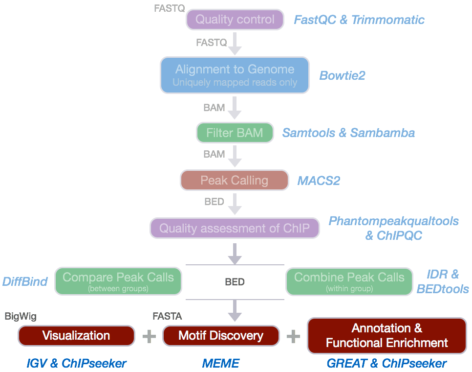
ChIPseeker is an R package for annotating ChIP-seq data analysis. It supports annotating ChIP peaks and provides functions to visualize ChIP peaks coverage over chromosomes and profiles of peaks binding to TSS regions. Comparison of ChIP peak profiles and annotation are also supported, and can be useful to estimate how well biological replications are. Several visualization functions are implemented to visualize the peak annotation and statistical tools for enrichment analyses of functional annotations.
Setting up
- Open up RStudio and open up the
chipseq-projectthat we created previously.
Note: If the desktop folder you had previously is no longer present, you can download a copy of the folder here.
- Open up a new R script (‘File’ -> ‘New File’ -> ‘Rscript’), and save it as
chipseeker.R
NOTE: This next section assumes you have the
ChIPseekerpackage installed as well as some additional dependencies, and minimally are using R 3.3.3. The desktops in the classroom have the latest version of ChIPseeker installed, for R 3.5.1, and we are using the latest version of ChIPseeker. For legacy versions of R use these instructions.
Otherwise, if you > are using the latest version of R you can run the following lines of code before proceeding.
if (!requireNamespace("BiocManager", quietly = TRUE))
    install.packages("BiocManager")
BiocManager::install("ChIPseeker", version = "3.8")
BiocManager::install("clusterProfiler", version = "3.8")
BiocManager::install("biomaRt", version = "3.8")
BiocManager::install("TxDb.Hsapiens.UCSC.hg19.knownGene", version = "3.8")
BiocManager::install("org.Hs.eg.db", version = "3.8")
BiocManager::install("BiocParallel", version = "3.8")
Getting data
As mentioned previously, these downstream steps should be performed on your high confidence peak calls. While we have a set for our subsetted data, this set is rather small and will not result in anything meaningful in our functional analyses. We have generated a set of high confidence peak calls using the full dataset. These were obtained post-IDR analysis, (i.e. concordant peaks between replicates) and are provided in BED format which is optimal input for the ChIPseeker package.
NOTE: the number of peaks in these BED files are are significantly higher than what we observed with the subsetted data replicate analysis.
We will need to copy over the appropriate files from Biocluster to our laptop.
You can do this using Cyberduck or MobaXterm (you can also use ‘scp’ or
similar from a Mac terminal).
Move over the BED files from Biocluster
(/home/classroom/hpcbio/chip-seq/idr-bed/*.bed) to your desktop. You will
want to copy these files into your chipseq-project into a
new folder called data/idr-bed.
Let’s start by loading the libraries. Type these into your ‘Source’ window in the script, then highlight the commands and select ‘Run’.
# Only needed for some Windows systems
library(BiocParallel)
register(SerialParam())

library(ChIPseeker)
library(TxDb.Hsapiens.UCSC.hg19.knownGene)
library(clusterProfiler)
library(biomaRt)
Now let’s load all of the data. As input we need to provide the names of our BED files in a list format.
# Load data
samplefiles <- list.files("data/idr-bed", pattern= ".bed", full.names=T)
samplefiles <- as.list(samplefiles)
names(samplefiles) <- c("Nanog", "Pou5f1")
What does samplefiles look like?
We also need to assign annotation databases generated from UCSC to a variable:
txdb <- TxDb.Hsapiens.UCSC.hg19.knownGene
NOTE: ChIPseeker supports annotating ChIP-seq data of a wide variety of species if they have transcript annotation TxDb object available. To find out which genomes have the annotation available follow this link and scroll down to “TxDb”. Also, if you are interested in creating your own TxDb object you will find more information here.
Visualization
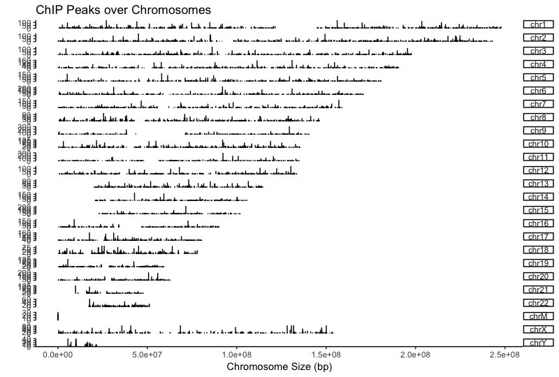
First, let’s take a look at peak locations across the genome. The covplot
function calculates coverage of peak regions across the genome and generates
a figure to visualize this across chromosomes. We do this for the Nanog peaks
and find a considerable number of peaks on all chromosomes.
# Assign peak data to variables
nanog <- readPeakFile(samplefiles[[1]])
pou5f1 <- readPeakFile(samplefiles[[2]])

# Plot covplot
covplot(nanog, weightCol="V5")
Using a window of +/- 1000bp around the TSS of genes we can plot the density of read count frequency to see where binding is relative to the TSS or each sample. This is similar to the plot in the ChIPQC report but with the flexibility to customize the plot a bit. We will plot both Nanog and Pou5f1 together to compare the two.
# Prepare the promotor regions
promoter <- getPromoters(TxDb=txdb, upstream=1000, downstream=1000)
Here it’s worth pausing to state what this next line is doing. Can anyone guess?
# Calculate the tag matrix
tagMatrixList <- lapply(samplefiles, getTagMatrix, windows=promoter)
# Profile plots
plotAvgProf(tagMatrixList, xlim=c(-1000, 1000), conf=0.95,resample=500, facet="row")
This may take a little time.
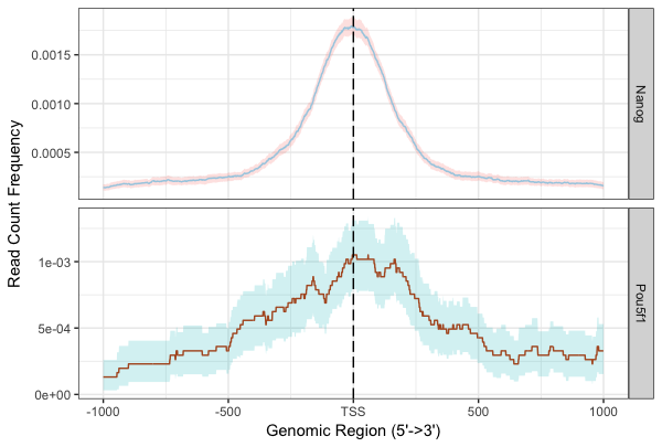
With these plots the confidence interval is estimated by bootstrap method (500 iterations) and is shown in the grey shading that follows each curve. The Nanog peaks exhibit a nice narrow peak at the TSS with small confidence intervals. Whereas the Pou5f1 peaks display a bit wider peak suggesting binding around the TSS with larger confidence intervals.
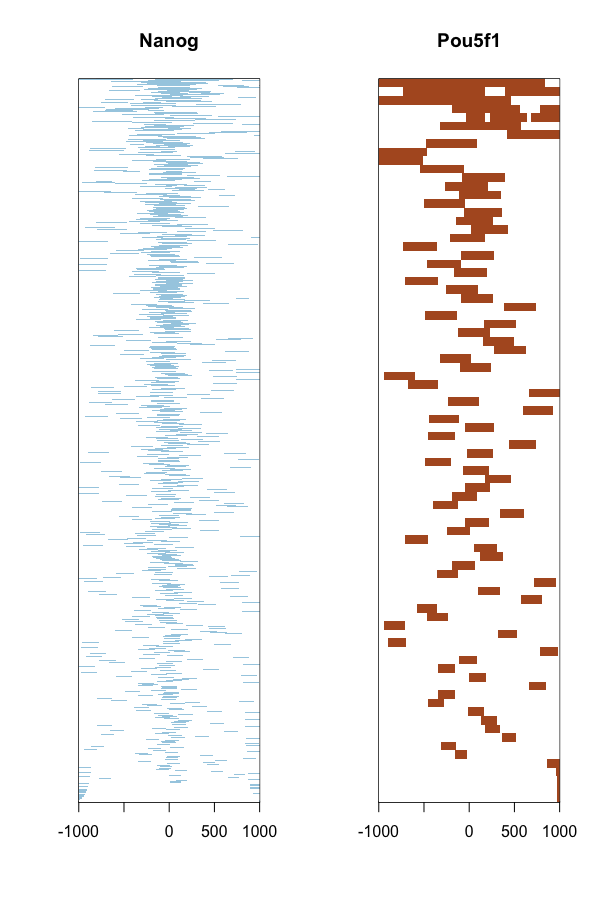
The heatmap is another method of visualizing the read count frequency relative to the TSS.
# Plot heatmap
tagHeatmap(tagMatrixList, xlim=c(-1000, 1000), color=NULL)
Annotation
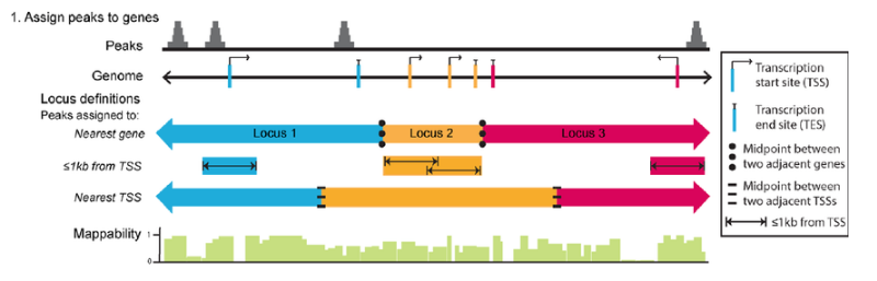
ChIPseeker implements the annotatePeak function for annotating peaks with
nearest gene and genomic region where the peak is located. Many annotation tools
calculate the distance of a peak to the nearest TSS and annotates the peak to
that gene. This can be misleading as binding sites might be located between
two start sites of different genes.
The annotatePeak function by default uses the TSS method, and provides
parameters to specify a max distance cutoff. There is also an option to report
ALL genes within this distance regardless of whether there is overlap with TSS
or not. For annotating genomic regions, annotatePeak function reports detail
information when genomic region is Exon or Intron. For instance, ‘Exon
(uc002sbe.3/9736, exon 69 of 80)’, means that the peak overlaps with the 69th
exon of the 80 exons that transcript uc002sbe.3 possess and the corresponding
Entrez gene ID is 9736.
Let’s start by retrieving annotations for our Nanog and Pou5f1 peaks calls:
# Get annotations
peakAnnoList <- lapply(samplefiles, annotatePeak, TxDb=txdb,
                       tssRegion=c(-1000, 1000), verbose=FALSE)
If you take a look at what is stored in peakAnnoList, you will see a summary
of genomic features for each sample:
# type 'peakAnnoList' at the R prompt in the console (command line) window

$Nanog
Annotated peaks generated by ChIPseeker
11023/11035  peaks were annotated
Genomic Annotation Summary:
             Feature  Frequency
9           Promoter 17.1731833
4             5' UTR  0.2358705
3             3' UTR  0.9706976
1           1st Exon  0.5443164
7         Other Exon  1.7781003
2         1st Intron  7.2121927
8       Other Intron 28.2318788
6 Downstream (<=3kb)  0.9434818
5  Distal Intergenic 42.9102785

$Pou5f1
Annotated peaks generated by ChIPseeker
3242/3251  peaks were annotated
Genomic Annotation Summary:
             Feature  Frequency
9           Promoter  3.7939543
4             5' UTR  0.1542258
3             3' UTR  1.0795805
1           1st Exon  1.3263418
7         Other Exon  1.6347933
2         1st Intron  7.4336829
8       Other Intron 30.9685379
6 Downstream (<=3kb)  0.9561999
5  Distal Intergenic 52.6526835
To visualize this annotation data ChIPseeker provides several functions. We will demonstrate a few using the Nanog sample only. We will also show how some of the functions can also support comparing across samples.
Some example simple visualizations
Let’s start with some simple summary visualization.
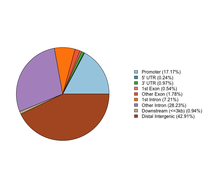
Pie chart of genomic region annotation
This plot gives overall categories, but it doesn’t account for instances where a peak may belong to multiple groups.
# Pie chart
plotAnnoPie(peakAnnoList[["Nanog"]])
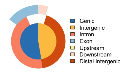
Vennpie of genomic region annotation
This is a version of the pie chart that does show additional layers, but still lacks some information.
# Venn pie
vennpie(peakAnnoList[["Nanog"]])
You can see overlaps here, but actual size of sets is hard to determine.
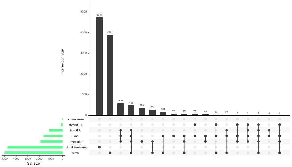
Upset Plot
Let’s generate an upset plot. This is another way to show intersections of sets, and is useful if you have more than three categories.
# Upset plot
upsetplot(peakAnnoList[["Nanog"]], sets.bar.color = "lightgreen")
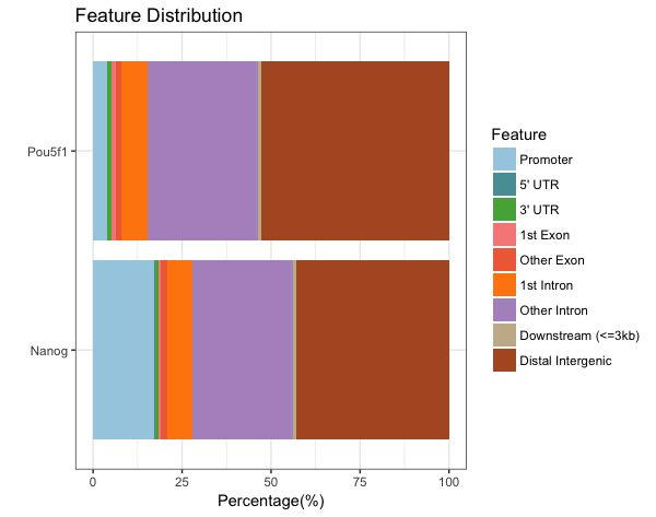
Barchart
We’ll run both Nanog and Pou5f1 here for comparison.
Here, we see that Nanog has a much larger percentage of peaks in promotor regions.
# Bar chart
plotAnnoBar(peakAnnoList)
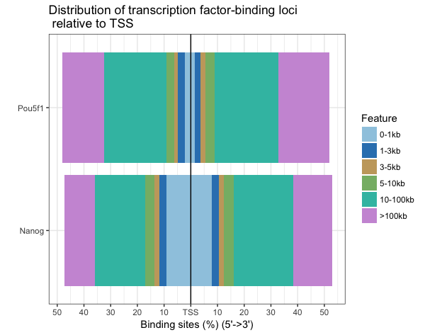
Distribution of TF-binding loci relative to TSS (multiple samples)
Nanog has also majority of binding regions falling in closer proximity to the TSS (0-10kb).
# Distance to TSS
plotDistToTSS(peakAnnoList, title="Distribution of transcription factor-binding loci \n relative to TSS")
Writing annotations to file
It would be nice to have the annotations for each peak call written to file, as
it can be useful to browse the data and subset calls of interest. The
annotation information is stored in the peakAnnoList object. To retrieve
it we use the following syntax:
# extract annotation
nanog_annot <- as.data.frame(peakAnnoList[["Nanog"]]@anno)
head(nanog_annot)
Take a look at this dataframe. You should see columns corresponding to your input BED file and addditional columns containing nearest gene(s), the distance from peak to the TSS of its nearest gene, genomic region of the peak and other information. Since some annotation may overlap, ChIPseeker has adopted the following priority in genomic annotation.
- Promoter
- 5’ UTR
- 3’ UTR
- Exon
- Intron
- Downstream (defined as the downstream of gene end)
- Intergenic
V4 and V5 are generic names R assigns to columns without IDs; these correspond to the peak name and peak weight.
One thing we don’t have is gene symbols listed in table. There are several ways to
get this information (e.g. using R’s OrganismDb annotation databases, like org.Hs.eg.db).
Here we’ll show a way to get this information using Biomart and add them to the table before we write to file. This makes it easier to browse through the results.
# Get entrez gene Ids
entrez <- nanog_annot$geneId

# Choose Biomart database
ensembl_genes <- useMart('ENSEMBL_MART_ENSEMBL',
                        host =  'www.ensembl.org')

# Create human mart object
human <- useDataset("hsapiens_gene_ensembl", ensembl_genes)

# Get entrez to gene symbol mappings
entrez2gene <- getBM(filters = "entrezgene",
                     values = entrez,
                     attributes = c("external_gene_name", "entrezgene"),
                     mart = human)
Here we do a bit of cleanup; we are matching the information in the table we get
back from biomart based on EntrezGene ID, then (if it’s defined) getting the
gene symbol, and finally gluing the information in the middle of the table with
cbind. We finally write to a tab-delimited file.
# Match the rows (gets a list of the position, or index, of match)
m <- match(nanog_annot$geneId, entrez2gene$entrezgene)

# Create a gene list, but check for no matches (NA); make this an empty string
# if no match
genesymbols <- ifelse(is.na(entrez2gene$external_gene_name[m]),
                      '',
                      entrez2gene$external_gene_name[m])

# Glue new table together, sticking the gene symbols in column 14
out <- cbind(nanog_annot[,1:13],
             geneSymbol=genesymbols,
             nanog_annot[,14:ncol(nanog_annot)])

# Write to file
write.table(out, file="results/Nanog_annotation.txt", sep="\t", quote=F, row.names=F)
Functional enrichment analysis
Once we have obtained gene annotations for our peak calls, we can perform functional enrichment analysis to identify predominant biological themes among these genes by incorporating knowledge from biological ontologies such as Gene Ontology, KEGG and Reactome.
Enrichment analysis is a widely used approach to identify biological themes. If you took the RNA-Seq workshop this may have been covered in great detail there. Once we have the gene list, it can be used as input to functional enrichment tools such as clusterProfiler (Yu et al., 2012), DOSE (Yu et al., 2015) and ReactomePA. We will go through a few examples here.
Single sample analysis
Let’s start with something we have seen before with RNA-seq functional analysis. We will take our gene list from Nanog annotations and use them as input for a GO enrichment analysis.
# Run GO enrichment analysis
ego <- enrichGO(gene = entrez,
                    keyType = "ENTREZID",
                    OrgDb = 'org.Hs.eg.db',
                    ont = "BP",
                    pAdjustMethod = "BH",
                    qvalueCutoff = 0.05,
                    readable = TRUE)

# Output results from GO analysis to a table
cluster_summary <- data.frame(ego)
write.csv(cluster_summary, "results/clusterProfiler_Nanog.csv")
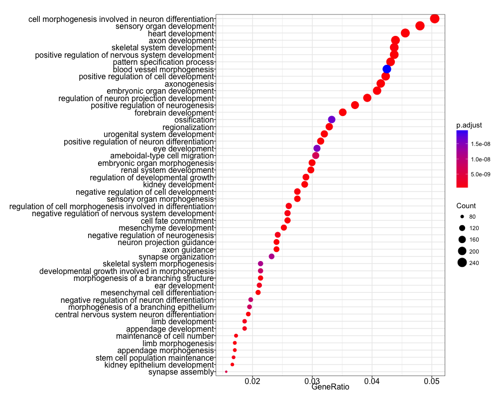
We can visualize the results using the dotplot function. We find many terms
related to development and differentiation and amongst those in the bottom
half of the list we see ‘stem cell population maintenance’. Functionally, Nanog
blocks differentiation. Thus, negative regulation of Nanog is required to
promote differentiation during embryonic development. Recently, Nanog has been
shown to be involved in neural stem cell differentiation which might explain the
abundance of neuro terms we observe.
# Dotplot visualization
dotplot(ego, showCategory=50)
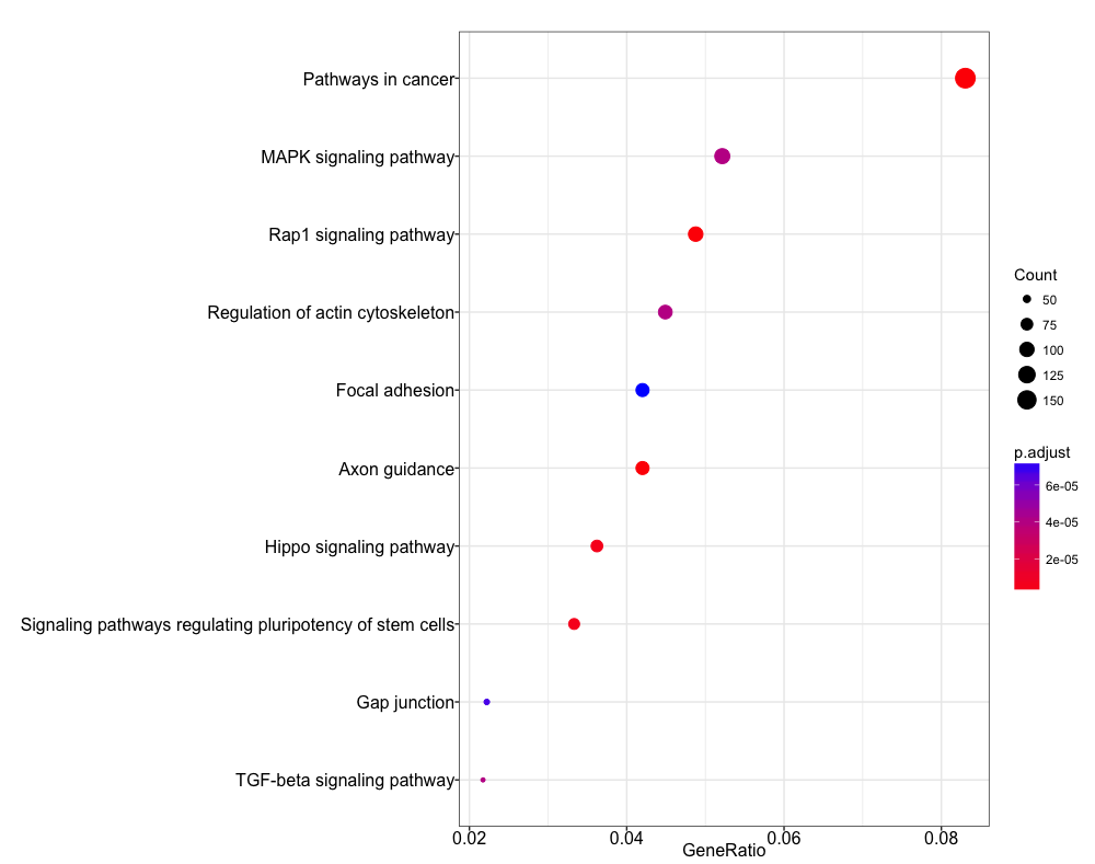
Let’s try a KEGG pathway enrichment and visualize again using the the dotplot. Again, we see a relevant pathway ‘Signaling pathways regulating pluripotency of stem cells’.
# Run KEGG enrichment analysis
ekegg <- enrichKEGG(gene = entrez,
                 organism = 'hsa',
                 pvalueCutoff = 0.05)

dotplot(ekegg)
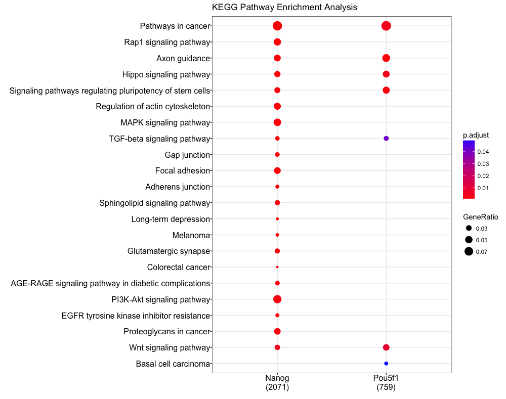
Multiple samples
Our dataset consist of two different transcription factor peak calls, so it
would be useful to compare functional enrichment results from both. We will do
this using the compareCluster function. We see similar terms showing up, and
in particular the stem cell term is more significant (and a higher gene ratio)
in the Pou5f1 data.
# Create a list with genes from each sample
genes = lapply(peakAnnoList, function(i) as.data.frame(i)$geneId)

# Run KEGG analysis
compKEGG <- compareCluster(geneCluster = genes,
                         fun = "enrichKEGG",
                         organism = "human",
                         pvalueCutoff  = 0.05,
                         pAdjustMethod = "BH")
dotplot(compKEGG, showCategory = 20, title = "KEGG Pathway Enrichment Analysis")
We have only scratched the surface here with functional analyses. Since the data is compatible with many current R packages for functional enrichment the possibilities there is a lot of flexibility and room for customization. For more detailed analysis we encourage you to browse through the ChIPseeker vignette and the clusterProfiler vignette.
This lesson has been developed by members of the teaching team at the Harvard Chan Bioinformatics Core (HBC). These are open access materials distributed under the terms of the Creative Commons Attribution license (CC BY 4.0), which permits unrestricted use, distribution, and reproduction in any medium, provided the original author and source are credited.